一文读懂 Pytorch 中的 Tensor View 机制

极市导读
本文主要内容是,通过图文结合的方式向读者讲解Pytorch的view 机制的原理。 >>加入极市CV技术交流群,走在计算机视觉的最前沿
前言
用户在使用 Pytorch 的过程中,必然会接触到 view 这个概念,可能会有用户对它背后的实现原理感兴趣。Pytorch 通过 view 机制可以实现 tensor 之间的内存共享。而 view 机制可以避免显式的数据拷贝,因此能实现快速且内存高效的比如切片和 element-wise 等操作。全文约 ~4000字&多图预警。
什么是 View
搬运官网的例子 https://pytorch.org/docs/stable/tensor_view.html#tensor-views: 在 Pytorch 中对一个张量调用 .view 方法,得到新的张量和原来的张量是共享内部数据的:
>>> t = torch.rand(4, 4)
>>> b = t.view(2, 8)
# `t` 和 `b` 共享底层数据
>>> t.storage().data_ptr() == b.storage().data_ptr()
True
# 对 view 之后的张量做修改也会影响到原来的张量
>>> b[0][0] = 3.14
>>> t[0][0]
tensor(3.14)
一般来说,Pytorch 中调用 op 会为输出张量开辟新的存储空间,来保存计算结果。但是对于支持 view 的 op 来说,输出和输入是共享内部存储的,在op计算过程中不会有数据的拷贝操作。op 的计算过程只是在推导输出张量的属性,而输入和输出的却别就只是对同一段内存的解析方式不同。还有一点需要注意的是,Pytorch 中 tensor 还有内存连续和不连续的概念。一般的 tensor 都是连续的,而 view op 则可能会产生内存非连续的 tensor,以 transpose op 为例:
>>> base = torch.tensor([[0, 1],[2, 3]])
>>> base.is_contiguous()
True
# transpose 是 view op
# 所以这里没有产生数据搬运
>>> t = base.transpose(0, 1)
# view op 产生的张量可能是不连续的
>>> t.is_contiguous()
False
# 而通过调用张量的 `.contiguous()` 方法
# 可以得到一个新的内存连续的张量
# 但是会产生数据搬运
>>> c = t.contiguous()
而要更好的理解 contiguous ,就需要先理解 tensor 的 stride 这个属性的含义。
tensor 的 stride 属性
我们知道 tensor 内部实际上是以一维数组的形式保存数据的,而在访问高维 tensor 数据的时候,内部就需要根据高维索引计算来对应的一维数组索引。以 4 维张量(shape = [2, 3, 4, 5])为例,假设现在要顺序打印该张量的每一个元素,下面用代码展示如何计算一维数组的索引:
import torch
arr = torch.rand(2, 3, 4, 5)
arr_1d = arr.flatten()
for d1 in range(2):
    for d2 in range(3):
        for d3 in range(4):
            for d4 in range(5):
                index = d1 * 3 * 4 * 5 + d2 * 4 * 5 + d3 * 5 + d4 * 1
                print(arr_1d[index])
可以看到在计算一维数组索引的时候,每次都有重复的计算,我们把这些重复计算的部分提取出来:
arr = torch.rand(2, 3, 4, 5)
arr_1d = arr.flatten()
s4 = 1
s3 = 5 * 1
s2 = 4 * 5 * 1
s1 = 3 * 4 * 5 * 1

for d1 in range(2):
    for d2 in range(3):
        for d3 in range(4):
            for d4 in range(5):
                index = d1 * s1 + d2 * s2 + d3 * s3 + d4 * s4
                print(arr_1d[index])
`

`s1, s2, s3, s4`  其实就是相当于 tensor 的 `stride` 属性。而张量 `arr` 的 `stride` 就等于 `[60, 20, 5, 1]`,打印验证一下:

`>>> import torch
>>> arr = torch.rand(2, 3, 4, 5)
>>> arr.stride()
(60, 20, 5, 1)
所以可知,stride 可以更高效的计算一维数组的索引,其每一维与 shape 一一对应。其含义就是在遍历某一维的时候,该维度索引加1 对应到在一维数据上的移动步长。
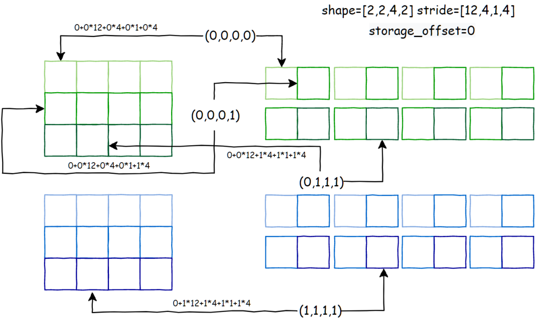
stride 图解
上图展示了一个三维张量 shape=[2,3,5] stride=[15,5,1] 。我们以多维索引 (d1=0, d2=0, d3=2) 为起点,展示当每一维索引+1的时候,对应到底层内存上的偏移量。
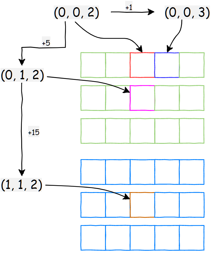
从上面的例子可以很清楚的看到,当每一维索引 +1 的时候,对应到内存上的偏移量就等于该维对应的 stride 大小。
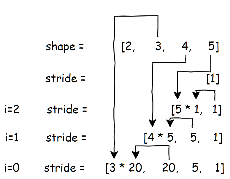
stride 计算方法
从上面的例子也可以得出 stride 的计算公式,假设张量维度是 n:
对应的代码实现:
arr = torch.rand(2, 3, 4, 5)
stride = [1] # 初始化第一个元素
# 从后往前遍历迭代生成 stride
for i in range(len(arr.shape)-2, -1, -1):
    stride.insert(0, stride[0] * arr.shape[i+1])
print(stride)       # [60, 20, 5, 1]
print(arr.stride()) # (60, 20, 5, 1)
图解算法流程:
以上是正常情况下,内存连续的 tensor 的 stride 的计算方式,如果正常方式计算得到的 stride 和 tensor 实际的 stirde 属性不一致的时候,就是非连续的 tensor 了。而除了 stride 和 shape 还有 storage_offset 这个属性也很关键 ,storage_offset 这个变量在下面介绍各个 view op 的时候会详细解释,表示张量在访问底层一维数据的时候,的起始偏移量,默认值是0。而 tensor view 机制的本质就是通过操作这三个属性,实现以不同的视角来解析同一段连续的内存。下一节,将会逐个解读 Pytorch 中常用的一些 tensor view 操作。通过代码结合图示的方式,展示上述三个属性是如何推导得到的。
常用的 5 个 View op 详解
1. diagonal
官方文档: https://pytorch.org/docs/stable/generated/torch.diagonal.html
该 op 的功能是,根据 offset,dim1和 dim2 这三个参数从 input 张量中取出对角元素。下面上图解释:
假设输入张量 shape=[2,4,4],接下来展示当固定 dim1=1, dim2=2 的时候, offset 参数的设置对输出结果的影响。
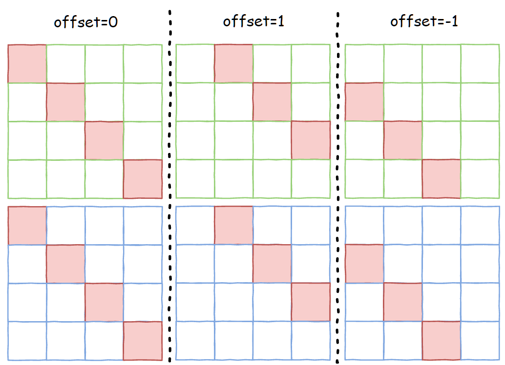
上图中红色填充部分就是当 offset 取不同值的时候,返回的张量实际所应该包含的数据。而 diagonal 是 view op,返回的输出张量是输入的一个 view,那么应该如何设置 offset 、shape 和 stride 这三个属性,使得输出张量只包含所需的结果而不产生实际的数据搬运呢?
属性推导细节
Pytorch 源码:https://github.com/pytorch/pytorch/blob/65f54bc000c4824a4e999ebfb6a27b252b696b0d/aten/src/ATen/native/TensorShape.cpp#L641**计算输出张量的 shape: **diagonal 输出大小的计算方式如下,首先移除输入 shape 的 dim1 和 dim2 维度,接着在剩下的 shape 末尾追加一维,大小是 diag_size,其计算伪代码如下:
 diag_size = max(min(input_shape[dim1], input_shape[dim2] - offset), 0)
else:
 diag_size = max(min(input_shape[dim1] + offset, input_shape[dim2]), 0)

output_shape = remove_dim1_and_dim2(input_shape).append(diag_size)
以上面图示的张量(shape=[2, 4, 4])为例:
# offset = 0
# diag_size = max(min(4, 4 - 0), 0) = 4
# output_shape = [2, diag_size]
>>> import torch
>>> arr = torch.rand(2, 4, 4).diagonal(0, 1, 2)
>>> arr.shape
torch.Size([2, 4])

# dim1 = 1, dim2 = 2
# offset = 1
# diag_size = max(min(4, 4 - 1), 0) = 3
# output_shape = [2, diag_size]
>>> import torch
>>> arr = torch.rand(2, 4, 4).diagonal(1, 1, 2)
>>> arr.shape
torch.Size([2, 3])

# dim1 = 1, dim2 = 2
# offset = -1
# diag_size = max(min(4 - 1, 4), 0) = 3
# output_shape = [2, diag_size]
>>> import torch
>>> arr = torch.rand(2, 4, 4).diagonal(1, 1, 2)
>>> arr.shape
torch.Size([2, 3])

# dim1 = 0, dim2 = 1
# offset = 0
# diag_size = max(min(2, 4 - 1), 0) = 2
# output_shape = [4, diag_size]
>>> import torch
>>> arr = torch.rand(2, 4, 4).diagonal(0, 0, 1)
>>> arr.shape
torch.Size([4, 2])
计算输出张量的 stride:stride 的计算和 shape 类似,都是先移除输入 stride 的 dim1 和 dim2 维度,接着接着在剩下的 stride 末尾追加一维,大小是 input_stride[dim1] + input_stride[dim2],其计算伪代码如下:
还是以上面图示的张量(shape=[2, 4, 4] stride=[16, 4, 1] )为例:
# offset = 0
# output_stride = [16, 4 + 1]
>>> import torch
>>> arr = torch.rand(2, 4, 4).diagonal(0, 1, 2)
>>> arr.stride()
torch.Size([2, 5])

# dim1 = 0, dim2 = 1
# offset = 0
# output_stride = [1, 16 + 4]
>>> import torch
>>> arr = torch.rand(2, 4, 4).diagonal(0, 0, 1)
>>> arr.stride()
torch.Size([1, 20])
计算输出张量的 storage_offset:storage_offset 的计算伪代码如下:
    storage_offset += offset * input_stride[dim2]
else:
    storage_offset -= offset * input_stride[dim1]
还是以上面图示的张量(shape=[2, 4, 4] stride=[16, 4, 1], storage_offset初始值为0 )为例:
# offset = 0
# storage_offset += 0 * input_stride[dim2] = 0

# dim1 = 1, dim2 = 2
# offset = 1
# storage_offset += 1 * input_stride[dim2] = 1

# dim1 = 1, dim2 = 2
# offset = -1
# storage_offset -= -1 * input_stride[dim1] = 4
接下来还是上图解释如何理解上面推导得到的三个输出属性吧。首先重新复习一下,顺序访问张量每个元素的时候,每个元素对应的一维索引计算代码:
# shape = [dim1, dim2, dim3, dim4]
# stride = [s1, s2, s3, s4]
for d1 in range(dim1):
 for d2 in range(dim2):
        for d3 in range(dim3):
            for d4 in range(dim4):
                id_index = storage_offset + d1 * s1 + d2 * s2 + d3 * s3 + d4 * s4
然后还是以张量(shape=[2, 4, 4] stride=[16, 4, 1] )为例,diagonal 参数为: offset=-1, dim1=1, dim2=2:
import numpy as np

arr = torch.rand(2, 4, 4)
diag_out = arr.diagonal(-1, 1, 2)

out_list = []
out_stride = [16, 5]
out_shape = [2, 3]
storage_offset = 4
arr_numpy = arr.flatten().numpy()
for d1 in range(2):
    for d2 in range(3):
        index = storage_offset + d1 * 16 + d2 * 5
        out_list.append(arr_numpy[index])

print(np.allclose(diag_out.numpy().flatten(), out_list))
# True
接下来以输出索引 (d1=0, d2=0) 为起点,展示当每一维索引+1的时候,对应到输入张量内存上的偏移量:
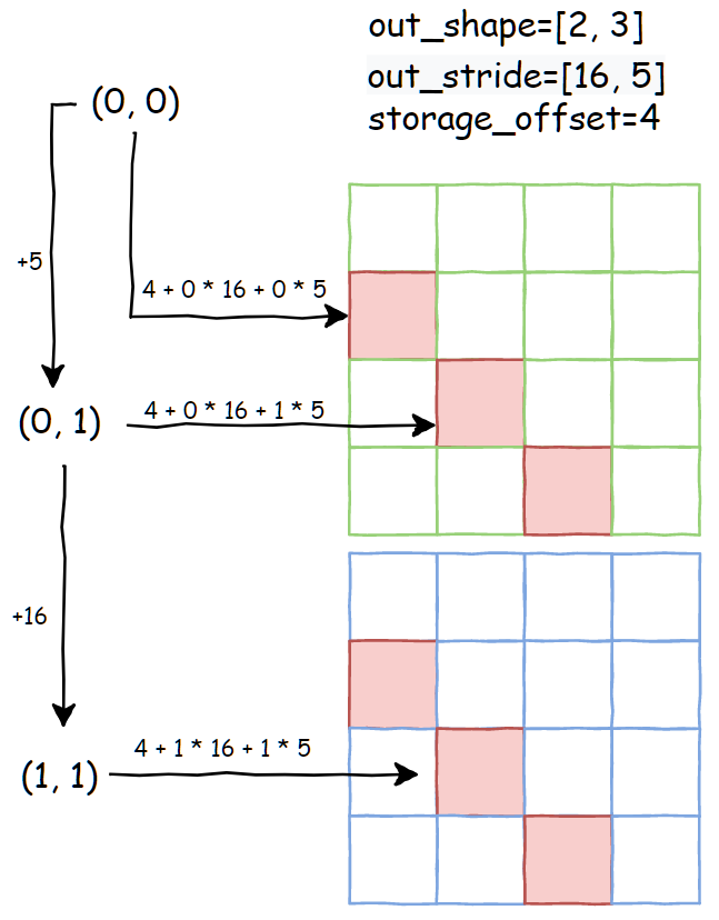
从上图就能清楚的看到,如何通过设置 storage_offset 、 shape 和 stride 着三个属性,来实现无内存拷贝的 diagonal 操作。而且可知 diagonal 产生的输出张量是非连续的,因为推导得到的 stirde=[16, 5],而如果是根据输出shape=[2, 3],其默认 stride=[3, 1],两者并不相等。连续调用 diagonal对一个张量连续调用 diagonal ,以上推导规则也是成立的。还是以 shape=[2,4,4] stride=[16, 4, 1] 张量为例:
import numpy as np

arr = torch.rand(2, 4, 4)
torch_out = arr.diagonal(-1, 1, 2)
# 第一个 digonal 的属性推导结果
# out_shape = [2, 3]
# out_stride = [16, 5]
# storage_offset = 4

torch_out2 = torch_out.diagonal(1, 0, 1)
# 第二个 digonal 的属性推导结果
# 是基于 torch_out 的属性推导
# out_shape = [2]
# out_stride = [16 + 5] = [21]
# storage_offset = 4 + 5 = 9

out_list = []
out_stride = [21]
out_shape = [2]
storage_offset = 9
arr_numpy = arr.flatten().numpy()
for d1 in range(2):
    index = storage_offset + d1 * 21
    out_list.append(arr_numpy[index])

print(np.allclose(torch_out2.numpy().flatten(), out_list))
还是以输出索引 (d1=0) 为起点,展示当每一维索引+1的时候,对应到输入张量内存上的偏移量:
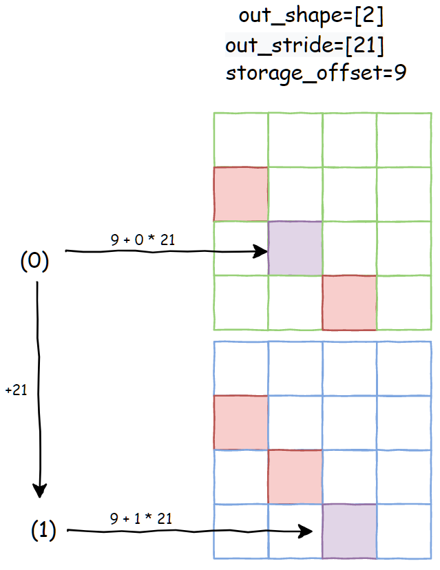
上图中,有颜色填充的都是第一次 diagonal 操作输出对应的数据,而第二次 diagonal 对应的就是紫色填充。
2. expand
官方文档: https://pytorch.org/docs/stable/generated/torch.Tensor.expand.html
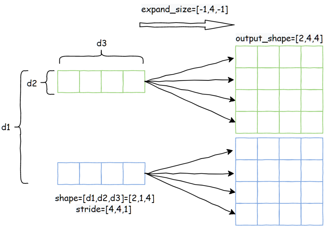
expand op 简单来说能实现将输入张量沿着大小为 1 的维度进行复制,复制的份数由第二个参数决定。关于 expand_size 的一些约定:
-
expand_size的长度大于等于输入张量,如果大于输入则输出相当于是增加了维度 -
对于输入张量为 1的维度,expand_size对应维度可以设置为大于等于1的值 -
对于输入张量不为 1的维度,expand_size对应维度只能设置为相等或者-1让算法自动推导 -
新添加的维度只能加在开头且不能设置 -1,相当于将整个输入张量进行复制
下面以张量 shape=[2, 1, 4] stride=[4, 4, 1] 为例,expand_size=[-1, 4, -1]:
属性推导:expand 推导输出张量属性的时候,直接继承输入的 storage_offset 。然后对于 shape 和 stride的推导分为两部分,分别是输出维度小于等于输入的部分,还有大于输入的部分。Pytorch 源码:https://github.com/pytorch/pytorch/blob/0a07488ed2c47765e337e290bd138c0e6e459cbd/aten/src/ATen/ExpandUtils.cpp#L47对于第一部分的计算伪代码,不考虑 expand_size 设置为 -1 的情况:
out_shape[i] = expand_size[i]
上面的代码说人话就是,对于原来是1的维度,如果对应的 expand_size 设置大于1, 则输出 stride设为0,读者可以思考一下,stride设为0其实就是等于复制。第二部分其实就更简单了:
out_shape[i] = expand_size[i]
也就是超出输入维度的部分,stride直接设置为 0 即可,因为新增的维度就是对整个张量进行复制。简单验证一下:
>>> arr = torch.rand(3,1,4)
>>> out = arr.expand(2,3,2,4)
>>> arr.shape
torch.Size([3, 1, 4])
>>> out.shape
torch.Size([2, 3, 2, 4])
>>> arr.stride()
(4, 4, 1)
>>> out.stride()
(0, 4, 0, 1)
最后还是以张量 shape=[2, 1, 4] stride=[4, 4, 1] 为例,当 expand_size=[2, 4, 4]的时候,推出 out_shape=[2, 4, 4] out_stride=[4,0,1] 。以输出索引 (d1=0, d2=0, d3=0) 为起点,展示当每一维索引+1的时候,对应到输入张量内存上的偏移量:
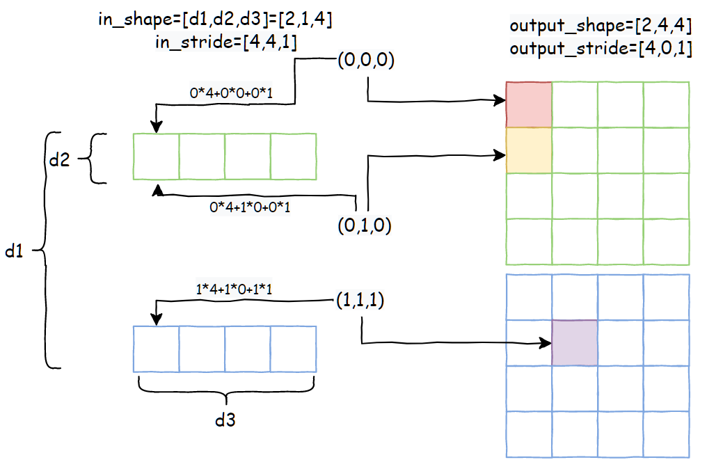
可以看到,通过合理设置 stride,就能实现无内存拷贝的 expand 操作。
3. narrow
官方文档:https://pytorch.org/docs/stable/generated/torch.narrow.html
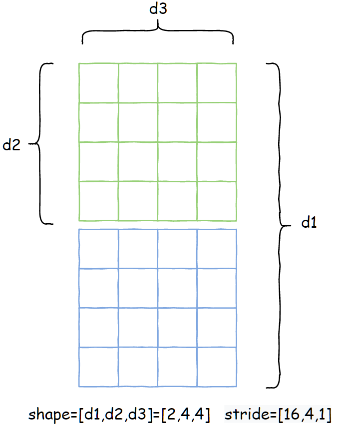
该 op 的功能是,对输入张量的 dim 维度进行截取,截取的长度为 length,起始索引是 start。以张量 shape=[2,4,4],stride=[16,4,1]为例,narrow 参数是 dim=1, start=1, length=2
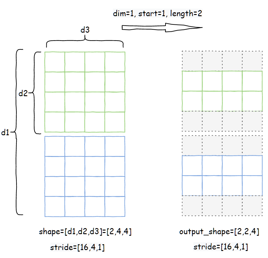
右边就是输出张量,灰色虚线部分相当于对于输出张量来说是不可见的。属性推导: Pytorch 源码:https://github.com/pytorch/pytorch/blob/65f54bc000c4824a4e999ebfb6a27b252b696b0d/aten/src/ATen/native/TensorShape.cpp#L909narrow的计算过程,只需要推导storage_offset 和 shape,stride直接沿用输入张量的 stride。storage_offset的计算方式:
也就是输出张量在读取内存的时候,加上的偏移量是 dim 维度的 stride 乘以 start,结合上图就很容易理解了。
4. permute
官方文档:https://pytorch.org/docs/stable/generated/torch.permute.html
该 op 的功能是将输入张量维度的顺序按照 dims 的值重新排列,且要求 len(dims)==len(input_tensor.shape)。下面以张量 shape=[2,3,4] stride=[12,4,1]为例,permute参数为 dims=(2,0,1):
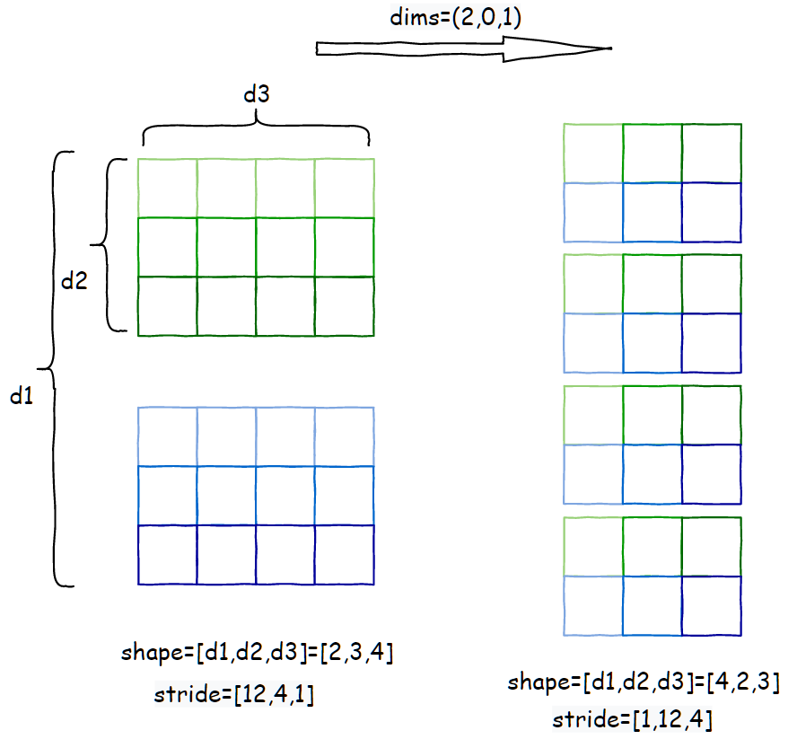
属性推导: Pytorch 源码:https://github.com/pytorch/pytorch/blob/65f54bc000c4824a4e999ebfb6a27b252b696b0d/aten/src/ATen/native/TensorShape.cpp#L927permute的属性推导规则也很简单,就是按照 dims的顺序,重新排列一下 shape 和 stride即可,storage_offset不变:
    out_shape[i] = in_shape[dims[i]]
    out_stride[i] = in_stride[dims[i]]
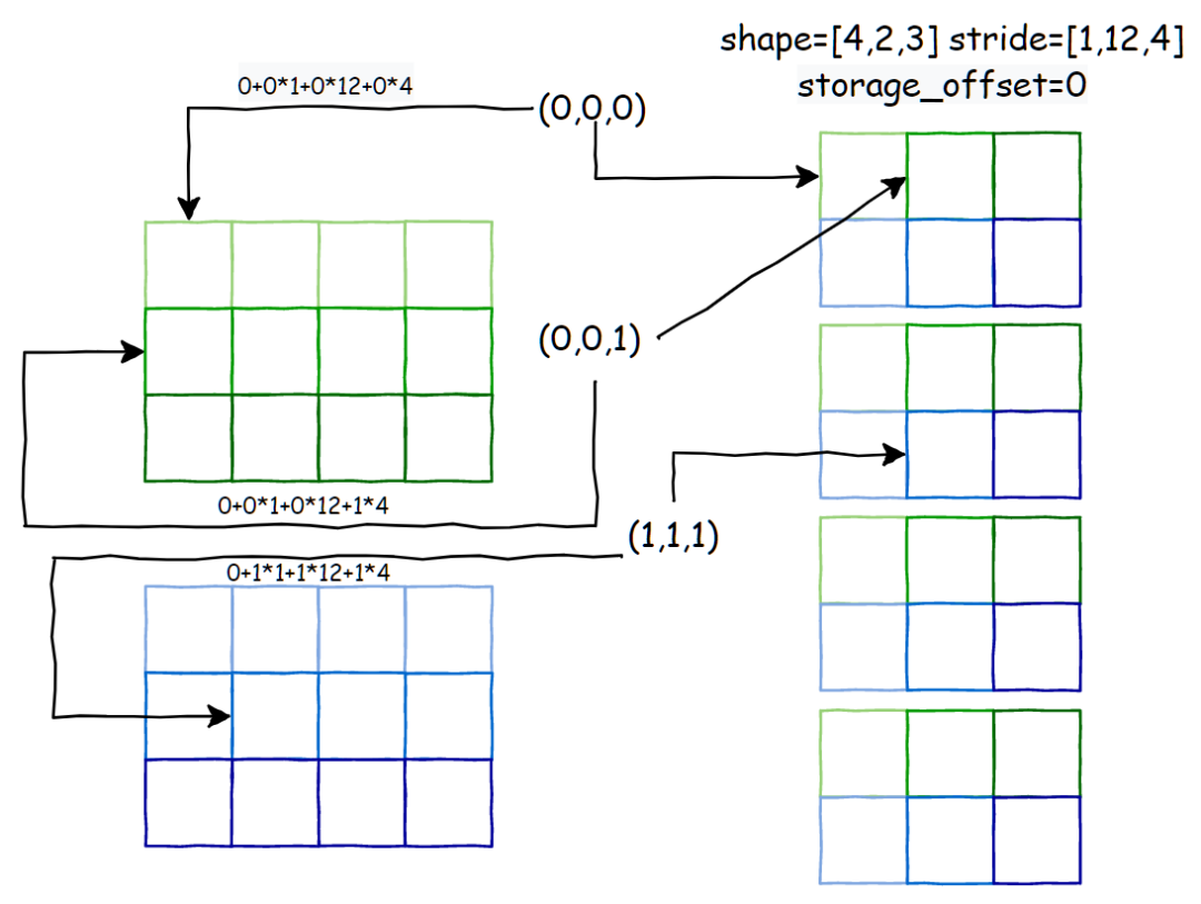
接下来以输出索引 (d1=0, d2=0, d3=0) 为起点,展示当每一维索引+1的时候,对应到输入张量内存上的偏移量:
5. unfold
官方文档:https://pytorch.org/docs/stable/generated/torch.Tensor.unfold.html
该 op 的功能是,将输入张量沿着 dimension 维度进行切片操作,每个分片大小是 size,分片之间的取值间隔是 step。简单来说就是在 dimension 维度有个大小是 size 的窗口,以 step 步长滑动取分片。输出张量的大小是,其他维度保持不变,dimension对应的维度变成 (dim - size) / step + 1,最后再添加一维,大小是size。以张量 shape=[2,3,4] stide=[12,4,1] 为例,unfold 参数 dimension=1, size=2, step=1:
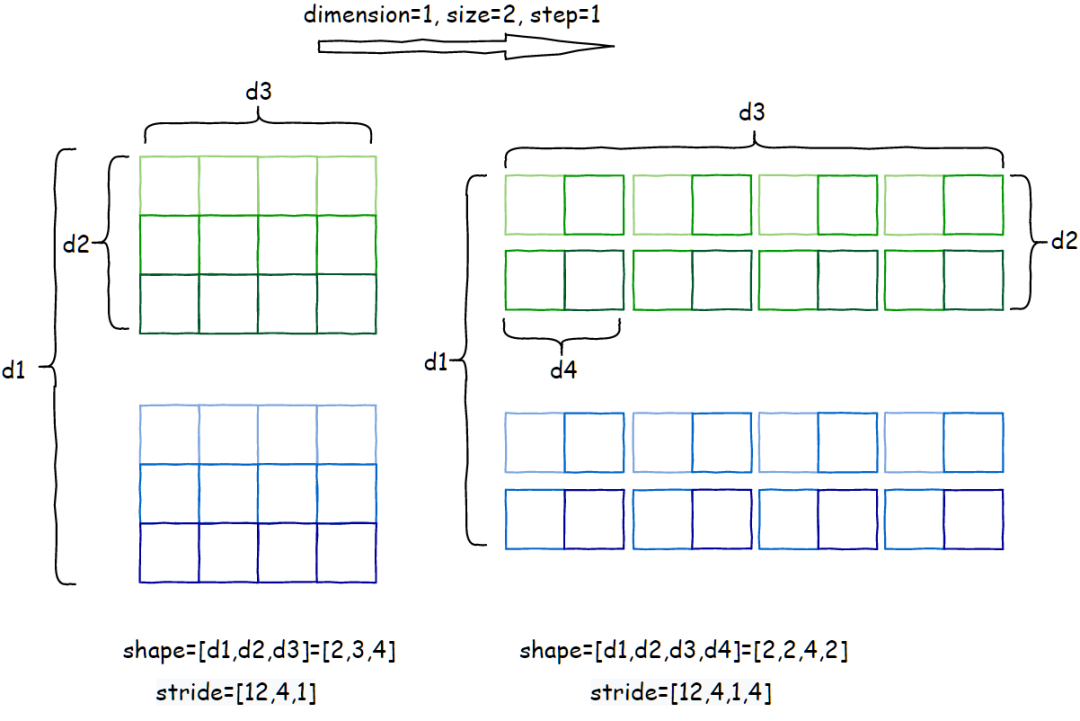
属性推导: Pytorch源码:https://github.com/pytorch/pytorch/blob/65f54bc000c4824a4e999ebfb6a27b252b696b0d/aten/src/ATen/native/TensorShape.cpp#L2242unfold的属性推导规则也很简单,storage_offset直接继承输入张量, shape 和 stride的推导伪代码:
out_shape = new array(out_dim)
out_stride = new array(out_dim)

# 末尾新增一维的推导规则
out_shape[out_dim-1] = size
out_stride[out_dim-1] = input_stride[dimension]

# 原来的维度推导
for d in range(len(input_shape)):
    self_size = input_shape[d];
    self_stride = input_stride[d];
    # dimension 对应维度推导规则
    if d == dimension:
      # 公式这样设置的原因是为了下取整
     out_shape[d] = (self_size - size) / step + 1
       out_stride[d] = step * self_stride
    # 非 dimension 维度直接继承输入属性
    else:
       out_shape[d] = self_size
       out_stride[d] = self_stride
接下来以输出索引 (d1=0, d2=0, d3=0,d4=0) 为起点,展示当每一维索引+1的时候,对应到输入张量内存上的偏移量:
总结
经过上面对常用 view op 的讲解,读者应该对 tensor view 机制可以有更深入的理解了~。不得不说这个 view 机制真的是很巧妙,能将看似在实现上没有关联的 op 统一到一起,实现上都变成只需要推导 storage_offset,shape和stride 这三个属性,无需内存拷贝。
参考资料
-
https://pytorch.org/docs/stable/tensor_view.html -
https://medium.com/swlh/deep-learning-with-pytorch-tensor-basics-part-1-stride-offset-contiguous-tensors-5d87476b7d9f
如果觉得有用,就请分享到朋友圈吧!
公众号后台回复“transformer”获取最新Transformer综述论文下载~

# CV技术社群邀请函 #

备注:姓名-学校/公司-研究方向-城市(如:小极-北大-目标检测-深圳)
即可申请加入极市目标检测/图像分割/工业检测/人脸/医学影像/3D/SLAM/自动驾驶/超分辨率/姿态估计/ReID/GAN/图像增强/OCR/视频理解等技术交流群
每月大咖直播分享、真实项目需求对接、求职内推、算法竞赛、干货资讯汇总、与 10000+来自港科大、北大、清华、中科院、CMU、腾讯、百度等名校名企视觉开发者互动交流~