基于图卷积文本模型的跨模态信息检索

【导读】近期专知将推出一系列小白入门自然语言处理问答方向的论文学习及相关代码的解析，本篇将介绍JingYu等的Modeling Text with Graph Convolutional Network for Cross-Modal Infomation Retrieval 的论文，以及tensorflow版的GCN开源代码。

作者：Jing Yu

翻译：Ying wang

00

摘要

作者针对跨模态信息检索的耦合特征学习提出了一个双路神经网络。其中的一路利用图卷积网络（GCN）进行基于图表示的文本建模，另一路使用具有非线性层的神经网络。这个模型通过训练成对相似性损失数来最大化匹配图文对的相似性，最小化不匹配对的相似性。实验显示，作者提出的模型表现出色，比目前最好模型精度提高了17%。

01

介绍

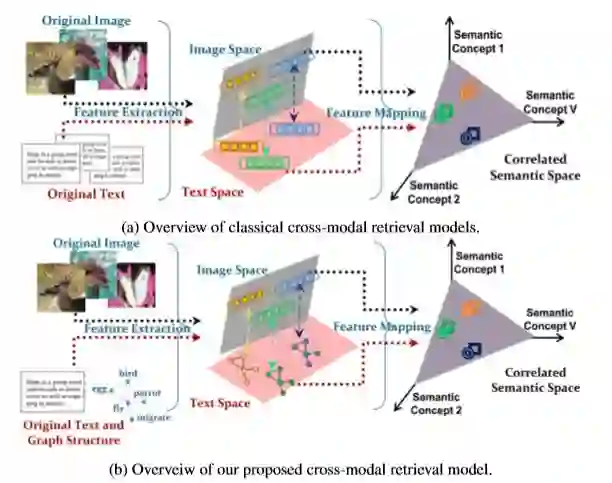
随着网络的发展，在线多媒体的信息越来越多样化，用户获取的信息可能存在于不同的模态中，对此，传统的单模式信息检索技术就显得格外苍白，人们就逐渐采用跨模态信息检索的技术。

特征表示是跨模型信息检索的基石。针对图片，作者采用卷积神经网络进行预训练获取数据特征；针对文本，作者在文章中提到采用vector-space模型来学习高维语义。然而，用字频向量表示文本的时候，却没有考虑词之间关系。研究者提出计算文本中所有词的word2vec向量的平均向量来表示文本。虽然这种词向量从相邻单词中获取更多信息，但它仍然忽略了文本中固有的全局结构信息，并且仅将该单词视为“flat”特征。

基于上述研究，为了获取文本词之间语义关系，作者采用图卷积(GCN)。基于GCN，作者提出了一个双路神经网络，被命名为 Graph-In-Network (GIN)，文本建模路径中采用GCN；图像建模路径中采用卷积神经网络，并采用成对相似性损失函数。

本文的主要工作有三点：

• 提出了一种跨模态检索模型，通过图卷积对文本数据进行建模，实现了不规则图结构数据与常规网格结构数据之间的跨模型检索

• 模型可以共同学习文本和图像特征以及图文相似性度量，并提供了一种端到端的训练模式

• 在4个数据集上结果显示，他们的模型优于现有的方法

02

方法

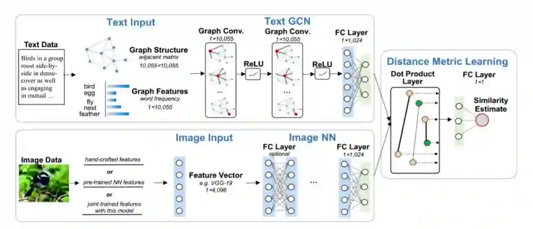
文本模型

文本建模中，有两个主要步骤，图结构 和GCN建模。

• Graph Construction:

通过特征图将结构信息与语义信息结合在一起。给定一组文本，从该语料库中获取words，并用W=[w1,w2,…,wn]表示，然后用预训练的word2vec嵌入表示。

我们用G=(V,E)来表示图结构，每个顶点v_i∈V对应一个词，每条边e_ij∈E 被定义为两字词之间的word2v-ec similarity：

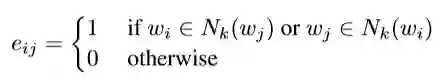
这里，Nk(w)表示K个最近邻居的集合，是通过计算词之间的word2vec嵌入的cosine的相似度。k是相邻参数的个数，试验中设置为8。图结构的参数用邻接矩阵A。

对于图特征，我们将每个文本用词袋向量表示，词的频率用一个一维向量表示。这样，就将结构信息（词的相似关系）跟语义信息（词向量表示）在一个特征图中结合起来了。

• GCN Modeling:

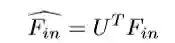
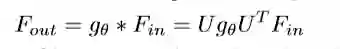
图卷积（GCN）将传统的卷积神经网络推广到不规则结构图中，这种思想基于图谱论。图卷积在频域作乘法处理，通过从频域到时域的逆变换获得特征图。假如给定一个文本，F_in表示图特征向量的输入，F_out表示图卷积输出向量。首先，F_in要经过傅里叶变换，这个变换基于图拉普拉斯的归一化，L=I_N-D^{-1/2}AD^{-1/2}   ，I_N 为单位矩阵， D为图结构G的度矩阵，A为邻接矩阵。L进行特征分解，L=UΛU^T , U为特征向量矩阵。Λ 为对角矩阵，其对角线上的元素为对应的特征值。对F_in进行傅里叶变换：

傅里叶逆变换为：

卷积计算用一个滤波器g_θ：

 [Defferrard et al., 2016] 提出了一个多项式滤波器g_θ:

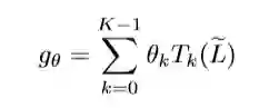
公式中，T_k(x)=2x*T_{k-1}(x)-T_{k-2}(x),  T_0(x)=1,  T_1(x)=x

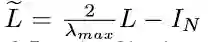
laibda_max为L的最大特征值，因此可以将卷积计算表示为F_out=g_θ*F_in 。对于一个文本，第i个图特征输入f_{in,i}∈F_in 指的是顶点vi 的词频，第i个特征的输出 f_{out,i}∈F_out表示为：

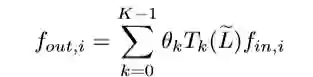
K作者在这里设置为3，就是卷积核的receptive filed，也就是说每次卷积会将中心顶点K-hop的特征进行加权求和。

作者提出的GCN模型中有2层图卷积，每层都采用ReLU激活函数，最后一层全连接层的维度与文本维度相同。

图模型

图模型中，作者采用了一组全连接层，经过实验发现，模型中仅保留最后一层没有进行特征微调的语义映射层效果最好。

目标函数

双路径模型（GIN）的最后一层，将前面两条路径的输出作为输入进行点乘运算，其输出为文本对的相似性分数。作者定义的损失函数，通过最大化匹配对的平均相似分数u+，最小化非匹配对的平均相似分数u- ,同时最小化匹配对的相似性分数的方差sigma^{2+} 和非匹配对的相似性分数方差sigma^{2-}， 将损失降到最小：

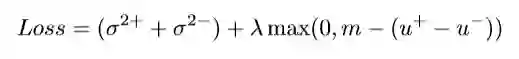
lamda,m 为参数，实验中分别为0.6，0.35。

文本Ti与图片Ii是同一类时：

文本Ti与图片Ii是不同类时：

其中，作者选择 Q1+Q2=200个文本对进行训练。

03

实验研究

数据集

作者分别在4个英文数据集（ English Wikipedia, NUS-WIDE, Pascal VOC, and TVGraz）以及中文 Wikipedia 数据集上进行实验。

实验

基于4个数据集，实验同时对比12个模型，对实验结果MAP进行评估。实验设置40000个图文匹配的正样本与40000个不匹配的负样本，dropout为0.2，学习率为0.001，Adam优化器，正则化0.005，参数lamda,m， 分别为0.6，0.35，进行50个epoch训练。

实验结果

• 文本查询图片实验中，在相同数据集上，GIN相比其他模型，MAP都要高，原因是模型通过图结构的形式表示出了词之间的语义关系。

• 图片查询文本的实验中，GIN似乎没有特别出色，原因在于作者采用的现成的图像特征向量，如果图像特征提取的神经网络用于模型中，实验结果会更好。

• 两组实验的平均MAP，GIN的结果相当好。
  

04

结论

作者提出的跨模态检索模型（GIN）将不规则图结构的文本表示与图像结合，共同学习特征和语义空间。经过实验并对比其他数据集，作者提出的模型具有更好的性能。

05

GCN开源代码解析

代码结构：

gcn

  ||_______init_.py       

  ||_______inits.py       #初始化工具

  ||_______layers.py    #定义模型层

  ||_______metrics.py  #评测指标，交叉熵损

                                    失与精确度

  ||_______models.py  #模型定义

  ||_______train.py      #训练代码

  ||_______utils.py      #辅助函数

utils.py 

从data文件中读取数据，文档中包含3组数据'cora', 'citeseer',与'pubmed'，每组数据有8种类型。'x'为训练数据的特征向量，'tx'为测试数据的特征向量，'allx'为所有训练数据的特征向量，'y'为训练数据的标签,'ty'为测试数据的标签，'ally'为所有数据的标签，'index'为测试数据的ID，'graph'为图数据。

def load_data(dataset_str):    """    Loads input data from gcn/data directory    ind.dataset_str.x => the feature vectors of the training instances as scipy.sparse.csr.csr_matrix object;    ind.dataset_str.tx => the feature vectors of the test instances as scipy.sparse.csr.csr_matrix object;    ind.dataset_str.allx => the feature vectors of both labeled and unlabeled training instances        (a superset of ind.dataset_str.x) as scipy.sparse.csr.csr_matrix object;    ind.dataset_str.y => the one-hot labels of the labeled training instances as numpy.ndarray object;    ind.dataset_str.ty => the one-hot labels of the test instances as numpy.ndarray object;    ind.dataset_str.ally => the labels for instances in ind.dataset_str.allx as numpy.ndarray object;    ind.dataset_str.graph => a dict in the format {index: [index_of_neighbor_nodes]} as collections.defaultdict        object;    ind.dataset_str.test.index => the indices of test instances in graph, for the inductive setting as list object.    All objects above must be saved using python pickle module.    :param dataset_str: Dataset name    :return: All data input files loaded (as well the training/test data).    """    names = ['x', 'y', 'tx', 'ty', 'allx', 'ally', 'graph']    objects = []    for i in range(len(names)):        with open("data/ind.{}.{}".format(dataset_str, names[i]), 'rb') as f:            if sys.version_info > (3, 0):                objects.append(pkl.load(f, encoding='latin1'))            else:                objects.append(pkl.load(f))
    x, y, tx, ty, allx, ally, graph = tuple(objects)    test_idx_reorder = parse_index_file("data/ind.{}.test.index".format(dataset_str))    test_idx_range = np.sort(test_idx_reorder)
    if dataset_str == 'citeseer':        # Fix citeseer dataset (there are some isolated nodes in the graph)        # Find isolated nodes, add them as zero-vecs into the right position        test_idx_range_full = range(min(test_idx_reorder), max(test_idx_reorder)+1)        tx_extended = sp.lil_matrix((len(test_idx_range_full), x.shape[1]))        tx_extended[test_idx_range-min(test_idx_range), :] = tx        tx = tx_extended        ty_extended = np.zeros((len(test_idx_range_full), y.shape[1]))        ty_extended[test_idx_range-min(test_idx_range), :] = ty        ty = ty_extended
    features = sp.vstack((allx, tx)).tolil()    features[test_idx_reorder, :] = features[test_idx_range, :]    adj = nx.adjacency_matrix(nx.from_dict_of_lists(graph))
    labels = np.vstack((ally, ty))    labels[test_idx_reorder, :] = labels[test_idx_range, :]
    idx_test = test_idx_range.tolist()    idx_train = range(len(y))    idx_val = range(len(y), len(y)+500)
    train_mask = sample_mask(idx_train, labels.shape[0])    val_mask = sample_mask(idx_val, labels.shape[0])    test_mask = sample_mask(idx_test, labels.shape[0])
    y_train = np.zeros(labels.shape)    y_val = np.zeros(labels.shape)    y_test = np.zeros(labels.shape)    y_train[train_mask, :] = labels[train_mask, :]    y_val[val_mask, :] = labels[val_mask, :]    y_test[test_mask, :] = labels[test_mask, :]
    return adj, features, y_train, y_val, y_test, train_mask, val_mask, test_mask

# 特征归一化并转换成元组模式def preprocess_features(features):    """Row-normalize feature matrix and convert to tuple representation"""    rowsum = np.array(features.sum(1))    r_inv = np.power(rowsum, -1).flatten()    r_inv[np.isinf(r_inv)] = 0.    r_mat_inv = sp.diags(r_inv)    features = r_mat_inv.dot(features)    return sparse_to_tuple(features)    # 设计计算公式 $D={1/2}(A+I)D^{-1/2}$def normalize_adj(adj):    """Symmetrically normalize adjacency matrix."""    adj = sp.coo_matrix(adj)    rowsum = np.array(adj.sum(1))    d_inv_sqrt = np.power(rowsum, -0.5).flatten()    d_inv_sqrt[np.isinf(d_inv_sqrt)] = 0.    d_mat_inv_sqrt = sp.diags(d_inv_sqrt)    return adj.dot(d_mat_inv_sqrt).transpose().dot(d_mat_inv_sqrt).tocoo()    def preprocess_adj(adj):    """Preprocessing of adjacency matrix for simple GCN model and conversion to tuple representation."""    adj_normalized = normalize_adj(adj + sp.eye(adj.shape[0]))    return sparse_to_tuple(adj_normalized)# 定义切比雪夫多项式def chebyshev_polynomials(adj, k):    """Calculate Chebyshev polynomials up to order k. Return a list of sparse matrices (tuple representation)."""    print("Calculating Chebyshev polynomials up to order {}...".format(k))
    adj_normalized = normalize_adj(adj)    laplacian = sp.eye(adj.shape[0]) - adj_normalized    largest_eigval, _ = eigsh(laplacian, 1, which='LM')    scaled_laplacian = (2. / largest_eigval[0]) * laplacian - sp.eye(adj.shape[0])
    t_k = list()    t_k.append(sp.eye(adj.shape[0]))    t_k.append(scaled_laplacian)
    def chebyshev_recurrence(t_k_minus_one, t_k_minus_two, scaled_lap):        s_lap = sp.csr_matrix(scaled_lap, copy=True)        return 2 * s_lap.dot(t_k_minus_one) - t_k_minus_two
    for i in range(2, k+1):        t_k.append(chebyshev_recurrence(t_k[-1], t_k[-2], scaled_laplacian))
    return sparse_to_tuple(t_k)

models.py

定义了一个model基类，以及两个继承自model类的MLP、GCN类

# 定义Model基类class Model(object)
# 定义MLP:class MLP(Model)
# 定义两层GCN， 采用交叉行损失与正则项class GCN(Model)

layer.py

定义Layers基类，以及两个继承自Layers类的Dense类和GCN类

# 定义一个layer基类class Layer(object)
# 定义Dense Layer 类class Dense(Layer)
# 定义GCN类，下面代码shi实现公式$D^{-1}AXW+b$class GraphConvolution(Layer):    """Graph convolution layer."""    def __init__(self, input_dim, output_dim, placeholders, dropout=0.,                 sparse_inputs=False, act=tf.nn.relu, bias=False,                 featureless=False, **kwargs):        super(GraphConvolution, self).__init__(**kwargs)
        if dropout:            self.dropout = placeholders['dropout']        else:            self.dropout = 0.
        self.act = act        self.support = placeholders['support']        self.sparse_inputs = sparse_inputs        self.featureless = featureless        self.bias = bias
        # helper variable for sparse dropout        self.num_features_nonzero = placeholders['num_features_nonzero']
        with tf.variable_scope(self.name + '_vars'):            for i in range(len(self.support)):                self.vars['weights_' + str(i)] = glorot([input_dim, output_dim],                                                        name='weights_' + str(i))            if self.bias:                self.vars['bias'] = zeros([output_dim], name='bias')
        if self.logging:            self._log_vars()
    def _call(self, inputs):        x = inputs
        # dropout        if self.sparse_inputs:            x = sparse_dropout(x, 1-self.dropout, self.num_features_nonzero)        else:            x = tf.nn.dropout(x, 1-self.dropout)
        # convolve        supports = list()        for i in range(len(self.support)):            if not self.featureless:                pre_sup = dot(x, self.vars['weights_' + str(i)],                              sparse=self.sparse_inputs)            else:                pre_sup = self.vars['weights_' + str(i)]            support = dot(self.support[i], pre_sup, sparse=True)            supports.append(support)        output = tf.add_n(supports)
        # bias        if self.bias:            output += self.vars['bias']
        return self.act(output)

论文链接：

https://arxiv.org/abs/1802.00985v1

代码地址：

https://github.com/tkipf/gcn

-END-

专 · 知

专知，专业可信的人工智能知识分发，让认知协作更快更好！欢迎登录www.zhuanzhi.ai，注册登录专知，获取更多AI知识资料！

欢迎微信扫一扫加入专知人工智能知识星球群，获取最新AI专业干货知识教程视频资料和与专家交流咨询！

请加专知小助手微信（扫一扫如下二维码添加），加入专知人工智能主题群，咨询技术商务合作~

专知《深度学习:算法到实战》课程全部完成！560+位同学在学习，现在报名，限时优惠！网易云课堂人工智能畅销榜首位！

点击“阅读原文”，了解报名专知《深度学习:算法到实战》课程