【论文笔记】通俗理解少样本文本分类 (Few-Shot Text Classification) (1)


Prior Knowledge
The knowledge of few-shot learning is NOT required. The only thing you need to know is that the general procedure of training neural networks and linear regression. You may notice that they used attentions. Please DO NOT worry what kind of attention they are using, I will explain it with a clear example.
The note includes:
- What problem is this work solving <--
- How to train the model (with a step-ty-step example) <--
- How to test the model (with a step-ty-step example)
- What attention is it using (with a step-ty-step example)

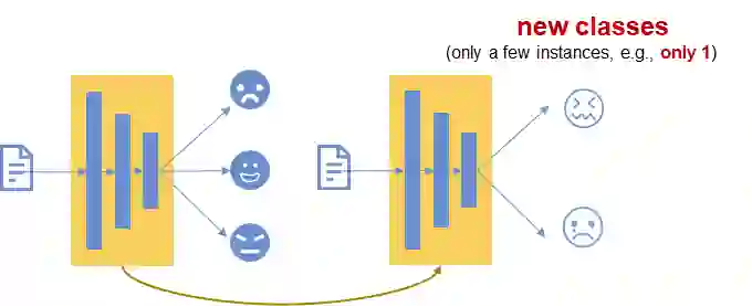
The situation is that we have many instances for some classes. But we only have a few (the most extreme case is only one) training instances for other classes.
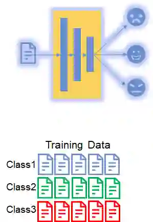
For example, let us say that we have 2 datasets. In the first dataset, we have 3 classes and each class has many instances for training a classifier. However, we do not have so much training instances for the other 2 totally different classes in the second dataset as shown below.
The research problem is that we have a model trained on the 1st dataset and whether this model can adapt quickly to the 2nd dataset. In other words, we will retrain the trained model based on the 2nd dataset and see if it will perform well in the case where we only have a few instances for training the 2 new classes.
You may think about using transfer learning. But based on the performance results in the paper, in this case, their method achieved much better performance than using transfer learning (Table 1 in the paper).
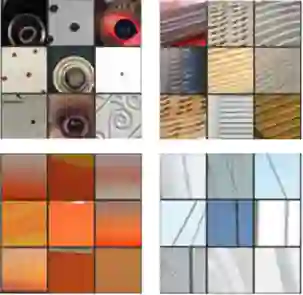
There is another thing worth mentioning is that solving this kind of problem might be easier in computer vision. Because the lower hidden layers are able to capture the low-level image features as shown below. However, for NLP tasks, it may be not so easy to capture such low-level features which can be generalised well to a new dataset.
All in all, the problem is how to train a model on a dataset that have many instances for each class and how to adapt this model to a new dataset which only has a few instances for each class. The classes in the new dataset are unseen in the first one.

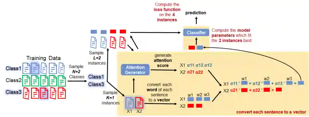
In this section, we will focus on how to train the model by using the 1st dataset. As shown in the Figure below, there are 3 classes in the dataset.
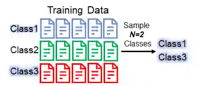
Step 1:
We sample N classes from all the classes in the dataset. (Please note: here we use N=2 just for the purpose of demonstrating. It doesn't mean in practice N=2 is a good setting. Please find how many classes exactly sampled in their paper.)
Step 2:
For each class sampled previously, we sample K instances. The K instances are named support set in the paper. (Please note again: here we use K=1 just for the purpose of demonstrating!)
Step 3:
We convert each word in each sentence to a vector (i.e., word embedding). In this example, the instance x1 has 3 words while the x2 has 2 words.
Step 4:
In this step, we take as input the sampled instances of an Attention Generator. The output of this generator is the attention scores of words. The score indicates the importance of each word in an instance.
We can safely SKIP the details of the Attention Generator since we will describe it later. For now, we can keep in mind that the output of this generator is attention scores.
Step 5:
Next, we calculate the weighted sum of the word embedding, by using the attention scores.
To summarise what we did so far, what we did is actually just converting an instance (e.g., a sentence) to a vector.
Step 6:
We feed the K=2 sentence vectors to a classifier. And we compute the model parameters which fit the 2 instances best. Because the classifier is a ridge regressor. Since we can find an analytical solution of the optimal parameters for a ridge regressor, the values of best parameters can be obtained immediately.
If you don't understand what is a ridge regressor, you can simply google or Baidu it. You will figure it out quickly as it is not a complicated model. HOWEVER, you can safely skip understanding what is it and go ahead with reading the next Steps.
Step 7:
At this point, we sample other L=2 instances for each sampled class. (Actually, in the sampling step, we sample totally L + K = 2 + 1 = 3 instances at the same time. And split them into 2 subsets. The set of K instances is called a support set mentioned in Step 2 and the set of L instances is called a query set.)
Please also note that setting L=2 is also just for demonstrating purpose. In practice, this number depends on your own case.
Step 8:
We run the same procedure as we did before to convert each instance to a vector.
Step 9:
We then feed these vectors to the classifier. Based on the predicted results, we compute the loss function (i.e., cross-entropy) on the instances in the query set and subsequently update the model parameters.
The model parameters here are actually the parameters in the Attention Generator. The reason is as follows:
Please note that the Attention Generator was used twice in each episode. We convert the K instances in the support set to vectors by utilising the Attention Generator. Next, these vectors are used to compute the analytical best parameters of the classifier. Then we convert the L instances in the query set to vectors by utilising the Attention Generator. We then compute the loss function based on the predicted results of the classifier. Therefore: 1) optimising the loss function involves the usage of Attention Generator twice on the support set and query set; 2) optimising the loss function is actually updating Attention Generator parameters. The classifier parameters can be solved analytically and computed by ourselves.
Based on the description above, you may observe that: one advantage of using the analytical solution of the classifier parameters is that we can learn the Attention Generator in an end-to-end manner by just optimising the cross-entropy loss function.
- Ending -
Running the whole process from Step 1 to 9 one time is called one episode. In the training phase, running multiple episodes are needed in practice.
Next: we will discuss how they adapt the model to and evaluate this model to a new dataset that includes new classes which are unseen in the old dataset.

