用LDA在R中聚类四本小说

作者：汪喵行  R语言中文社区专栏作者

知乎ID：https://www.zhihu.com/people/yhannahwang

前言

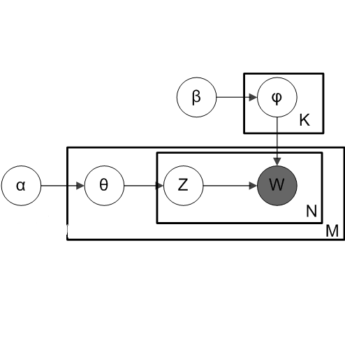
在文本挖掘里面，除了情感分析，还有一个很重要的主题就是topic modeling。在生活中，有时候对于文章进行分类时，如果用topic modeling的方法，会比人工分类有效率的多。在topic modeling中，最常用的方法就是LDA（Latent Dirichlet allocation）。简单来说，这种方法可以看成：

1.把每篇文章看作是topic的集合。比如对于一个双话题模型，我们可以认为文章1有90%的可能性是话题1，10%的可能性是话题2；

2.把每个话题（topic）看成是词的集合（bag of words），比如对于话题“政治”，里面会有“政府”，“国会”之类，对于“娱乐”这个话题，里面可能会包括“电影”等等。

我们选取了四本小说：《Twenty Thousand Leagues under the Sea》《The War of the Worlds》 《Pride and Prejudice 》《Great Expectations》，把四本小说的所有章节全部打乱，用这些章节来form 4 个topics。如果聚类的效果好的话，这4个topics应该是对应四本小说的。所以步骤是：

1. 首先把四本小说拆成章节并打乱去掉名字（相当于是unlabeled的凌乱的chapters），文本预处理

2.画四本小说的wordcloud

3.用这些章节去聚类4个topics

4.把所有章节带着小说名称放进4个topics里，看看我们的聚类效果如何

需要用到的packages: gutenbergr / topicmodels / Stringr / dplyr / wordcloud2 / ggplot2 / tidytext/tidyr

先library一遍

library(gutenbergr)    # for loading bookslibrary(topicmodels)   # for modeling topicslibrary(stringr)       # deal with stringlibrary(dplyr)         # do operations on table or dataframe (can do multiple operations using "%>%")library(wordcloud2)    # draw word cloudlibrary(ggplot2)       # draw pictureslibrary(tidytext)      # tidying model objects, extract topic-related probabilitieslibrary(tidyr)         # tidying model object

1.加载四本书并拆分成章节

#load the four bookstitles <- c("Twenty Thousand Leagues under the Sea", "The War of the Worlds","Pride and Prejudice", "Great Expectations")books <- gutenberg_works(title %in% titles) %>% gutenberg_download(meta_fields = "title")# split into chapters (with no book titles)chapters <-   books %>% group_by(title) %>%             mutate(chapter = cumsum(str_detect(text, regex("^chapter ", ignore_ca              se = TRUE)))) %>%             ungroup() %>% filter(chapter > 0) %>%             unite(document, title, chapter)

Output:

可以看出，gutenberg_id代表了书名，text代表了书的内容，每一列都是自然行划分的句子。接下来我们要把它们分割成词语，去掉停用词（a,the之类），因为这些停用词对于我们最后的聚类分析没有意义并且影响结果。然后计算每一个chapter里的每个词语的频数。

# split into wordschapters_word <- chapters %>% unnest_tokens(word, text)# remove stop words & find document-word countswordcount <- chapters_word %>% anti_join(stop_words) %>%            count(document, word, sort = TRUE) %>% ungroup()

Output:

其实就是每一个词语在每一个章节里出现的频数啦。

2 绘制四本书的wordcloud

首先把四本小说分清楚，并把每本小说全部分割成词语:

by_chapter1 <- books %>% group_by(title) %>% ungroup() %>% unite(document, title)# split into wordsby_chapter_word1 <- by_chapter1 %>% unnest_tokens(word, text)

以pride and prejudice为例:

#找出price and prejudice里的所有词word_countsPAP <- by_chapter_word1[by_chapter_word1$document=='Pride and Prejudice',]  #去掉停用词rept_PAP<- anti_join(word_countsPAP,stop_words)#按词频倒序排序nPAP <- as.data.frame(table(rept_PAP$word))nPAP <- nPAP[order(-nPAP$Freq),]#选取频率最高的前100个词top100PAP <- nPAP[c(1:100),]#画云图wordcloud2(top100PAP, rotateRatio = 1,color= "random-light",minRotation = -3.3/4, maxRotation = 3.3/4,size = 1.3)

其他三本的绘制云图的方法是一样的，就不放代码了，大家可以照这个例子，自己动手实践下。

3 用以上章节聚类4个Topics

#create a DocumentTermMatrixchapterDTM<- wordcount %>% cast_dtm(document, word, n)# set seed to trace backchapterLDA <- LDA(chapterDTM, k = 4, control = list(seed = 1234))

首先我们要生成一个DTM，因为LDA模型的input需要DTM，然后通过LDA（），根据词频。以章节为单元来生成topics： k=4说明我们要生成4个topics。

Output:

我们可以通过matrix='beta'这个参数来得到每个特定的词属于每一个topic的概率，如下：

(here "beta" represents the probablity that one certain word belongs to one certain topic)

# per-topic-per-word probabilities (beta)  _ one-topic-per-term-per-row formatchapter_topics <- tidy(chapterLDA, matrix = "beta")

Output：

我们想要得到每一个topic的前五个高频词并绘制出来：

相当于就是把四个topics分开，然后把每个topic下面的对应的所有词按照beta概率进行倒序排列，找到前五个概率（beta）最大的词语。

#find top-5 terms within each topictop_terms <- chapter_topics %>% group_by(topic) %>% top_n(5, beta) %>% ungroup() %>% arrange(topic, -beta)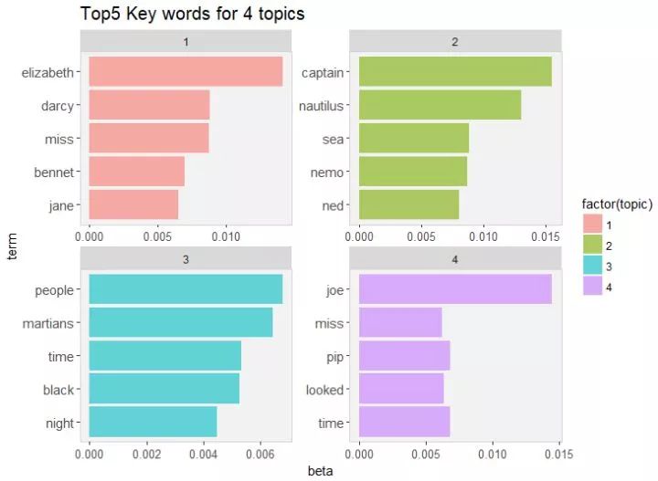

通过上图可以清晰看出这四个topic分别代表的是哪本小说。通过和上文小说的高频词进行比较，粗略上看，发现我们用unlabelled的章节进行聚类得到的四个topics和四本小说的相关度还是很高的。

4 把小说名字放进去，看看聚类效果

上面我们已经成功用打乱的章节聚类成了四本小说，通过topics的高频词和小说高频词的云图对的对比粗略得到模型结果还不错，但是具体聚类效果如何，可能需要我们把章节重新带着小说名称放进topics，看看被分错的章节多不多。

gamma 不同于beta，gamma这里代表的是每一个章节属于每一个topic的概率:

# check per-document-per-topic probabilities (gamma)chapters_gamma <- tidy(chapterLDA, matrix = "gamma")chapters_gamma <- chapters_gamma %>% separate(document, c("title", "chapter"), sep = "_", convert = TRUE)

Output:

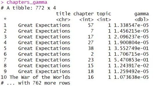
比如第一条，说明Great Expectation的第57章属于topic1的概率就是1.33857e-05.

把章节分回topics里:

chapter_classifications <- chapters_gamma %>% group_by(title, chapter) %>% top_n(1, gamma) %>% ungroup()

那么哪些章节被错分了呢？我们画个图会直观一些：

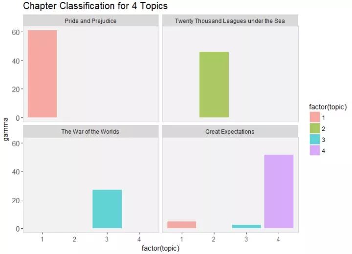
从图中可以看出，Great Expectation有几章被错误分到了topic1和topic2，我们要具体看一下到底是哪几章被分错了：

#find the misclassified chaptersmisclassifications <-  chapter_classifications %>%     inner_join(book_topics, by = "topic") %>%     filter(title != consensus)

Output:

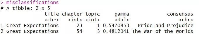
可以看出，Great Expectation的23章被错误分到了代表pride and prejudice的那个topic，Great Expectation的第54章被错误分到了代表 The war of the Worlds的topic里。

我们还想知道词被分到的topics的情况,所以把词也按照概率分到topic里面去:

# find which words in each document were assigned to which topicassignws <- augment(chapterLDA, data = chapterDTM)#combine book_topics and tableassigntopic <- assignws %>%separate(document, c("title", "chapter"), sep = "_", convert = TRUE) %>% inner_join(book_topics, by = c(".topic" = "topic"))

画出词被分的topic的情况：

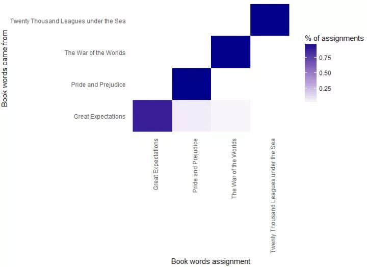
同样的，有些本来属于Great Expectation的词，错误分到了代表另外两本小说的topics里。

最后，哪些词是最容易被分错的呢？

#get wrong wordsmisclassified_word <- assigntopic %>% filter(title != consensus)misclassified_word %>% count(title, consensus, term, wt = count) %>% ungroup() %>% arrange(desc(n))

Output:

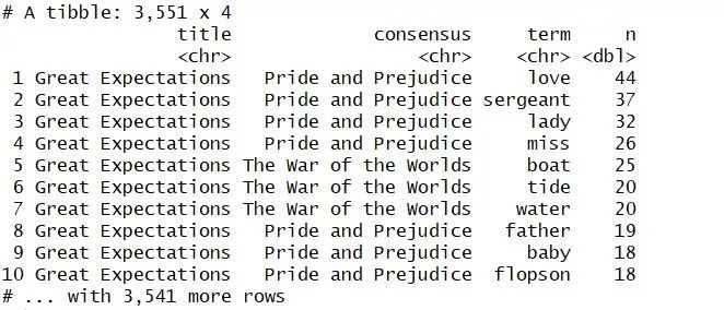
可以看出，"love","miss"这些词是最容易被分错的，这也很好理解，无论是哪种小说，里面出现love，miss这种词语的可能性确实是很高的。

总结：

Topic modeling不仅仅适合话题分类，也适合小说分类，通过clustering的方法，我们可以实现更快地给文本分类。

参考：

Text Mining with R

（https://www.tidytextmining.com/）

(附)

画图代码:

1.keywords for 4 topics:

top_terms %>% mutate(term = reorder(term, beta)) %>% ggplot(aes(term,beta,fill=factor(topic))) + geom_col(show.legend = TRUE,alpha = 0.6) + labs(title = "Top5 Key words for 4 topics")+ facet_wrap(~ topic, scales = "free") + coord_flip(expand = TRUE)+ theme(axis.text.y = element_text(size=11),       axis.text.x = element_text(size=10),       panel.grid.major=element_blank(),       panel.grid.minor=element_blank(),       panel.background = element_rect(fill = "gray95"),       panel.border=element_rect(fill="transparent",color="light gray"),       plot.title = element_text(lineheight = 610,colour = "black",size = 15))

2.chapter classification for 4 topics:

chapters_gamma %>% mutate(title = reorder(title, gamma * topic)) %>% ggplot(aes(factor(topic),fill=factor(topic), gamma)) + labs(title = "Chapter Classification for 4 Topics")+ theme(axis.text.y = element_text(size=11),       axis.text.x = element_text(size=10),       panel.grid.major=element_blank(),       panel.grid.minor=element_blank(),       panel.background = element_rect(fill = "gray95"),       panel.border=element_rect(fill="transparent",color="light gray"),       plot.title = element_text(lineheight = 610,colour = "black",size = 15))+ geom_col(show.legend = TRUE,alpha = 0.6) + facet_wrap(~ title)

3.words assigned to topics:

ssigntopic %>% count(title, consensus, wt = count) %>% group_by(title) %>% mutate(percent = n/sum(n) ) %>% ggplot(aes(consensus, title, fill = percent)) + geom_tile() + scale_fill_gradient2(high = "dark blue") + theme_minimal() + theme(axis.text.x = element_text(angle = 90, hjust = 1),       panel.grid = element_blank()) + labs(x = "Book words assignment",      y = "Book words came from",      fill = "% of assignments")

公众号后台回复关键字即可学习

回复 爬虫             爬虫三大案例实战  
回复 Python        1小时破冰入门

回复 数据挖掘      R语言入门及数据挖掘
回复 人工智能      三个月入门人工智能
回复 数据分析师   数据分析师成长之路 
回复 机器学习      机器学习的商业应用
回复 数据科学      数据科学实战
回复 常用算法      常用数据挖掘算法

我怎么这么好看