系列教程GNN-algorithms之二:《切比雪夫显神威—ChebyNet》
【导读】利用Chebyshev多项式拟合图卷积核应该是GCN中比较普遍的应用方法。Chebyshev多项式核主要解决了两个问题:1.经过公式推导变换不再需要特征向量的分解。2.通过Chebyshev的迭代定义降低了计算复杂度。本文将结合公式推导详细介绍基于tensorflow的ChebyNet实现。
系列教程《GNN-algorithms》
本文为系列教程《GNN-algorithms》中的内容,该系列教程不仅会深入介绍GNN的理论基础,还结合了TensorFlow GNN框架tf_geometric对各种GNN模型(GCN、GAT、GIN、SAGPool等)的实现进行了详细地介绍。本系列教程作者王有泽(https://github.com/wangyouze)也是tf_geometric框架的贡献者之一。
系列教程《GNN-algorithms》Github链接:
https://github.com/wangyouze/GNN-algorithms
TensorFlow GNN框架tf_geometric的Github链接:
https://github.com/CrawlScript/tf_geometric
前言
当GCN如日中天的时候,大部分人并不知道GCN其实是对ChebyNet的进一步简化与近似,ChebyNet与GCN都属于谱域上定义的图卷积网络。本教程将教你如何用Tensorflow构建ChebyNet模型进行节点分类任务。完整的代码可在Github中下载:
https://github.com/CrawlScript/tf_geometric/blob/master/demo/demo_chebynet.py.
ChebyNet简介
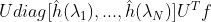
由图上的傅里叶变换公式我们可以得到卷积核h在图f上的卷积公式:

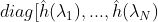
第一代GCN中简单把
中的对角线元素
替换为参数
,此时的GCN就变成了这个样子:
但是这样问题很多,如:
图卷积核参数量大,参数量与图中的节点的数量相同。
卷积核是全局的。
运算过程涉及到特征分解,复杂度高。
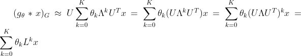
为了克服以上问题,第二代GCN进行了针对性的改进:用k阶多项式来近似卷积核:
将其代入到:
可以得到:
所以第二代GCN的卷积公式是:
第二代GCN直接对拉普拉斯矩阵进行变换,从而避免了特征分解这一耗时操作。
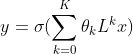
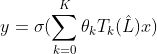
ChebyNet在第二代GCN的基础上用ChebyShev多项式展开对卷积核进行近似,即令:
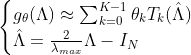
切比雪夫多项式的递归定义:
这样有两个好处:
1. 卷积核的参数从原先一代GCN中的n个减少到k个,从原先的全局卷积变为现在的局部卷积,即将距离中心节点k-hop的节点作为邻居节点。
2. 通过切比雪夫多项式的迭代定义降低了计算复杂度。
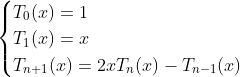
因此切比雪夫图卷积公式变为:


对上述推导过程不清楚的人可以参考我的博客:https://www.jianshu.com/p/35212baf6671
教程完整代码链接:https://github.com/CrawlScript/tf_geometric/blob/master/demo/demo_chebynet.py
论文地址:https://arxiv.org/pdf/1606.09375.pdf
教程目录
开发环境
ChebyNet的实现
模型构建
ChebyNet训练
ChebyNet评估
开发环境
操作系统: Windows / Linux / Mac OS
Python 版本: >= 3.5
依赖包:
tf_geometric(一个基于Tensorflow的GNN库)
根据你的环境(是否已安装TensorFlow、是否需要GPU)从下面选择一条安装命令即可一键安装所有Python依赖:
	pip install -U tf_geometric # 这会使用你自带的TensorFlow,注意你需要tensorflow/tensorflow-gpu >= 1.14.0 or >= 2.0.0b1

	pip install -U tf_geometric[tf1-cpu] # 这会自动安装TensorFlow 1.x CPU版

	pip install -U tf_geometric[tf1-gpu] # 这会自动安装TensorFlow 1.x GPU版

	pip install -U tf_geometric[tf2-cpu] # 这会自动安装TensorFlow 2.x CPU版

	pip install -U tf_geometric[tf2-gpu] # 这会自动安装TensorFlow 2.x GPU版
教程使用的核心库是tf_geometric,一个基于TensorFlow的GNN库。tf_geometric的详细教程可以在其Github主页上查询:
https://github.com/CrawlScript/tf_geometric
ChebyNet的实现
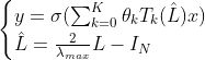
对图的邻接矩阵进行归一化处理得到拉普拉斯矩阵,归一化的方式有以下三种:
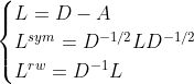
以及根据得到的归一化的拉普拉斯矩阵计算:
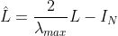
re-scaled特征值对角矩阵,将其变换到[-1,1]之间。具体实现请看chebynet_norm_edge的完整代码实现:
https://github.com/CrawlScript/tf_geometric/blob/master/tf_geometric/nn/conv/chebynet.py
num_nodes = x.shape[0]
norm_edge_index, norm_edge_weight = chebynet_norm_edge(edge_index, num_nodes, edge_weight, lambda_max, normalization_type=normalization_type)
利用切比雪夫多项式的迭代定义递推计算高阶项(节省了大量运算),最后输出模型结果,即多项式和:
    T0_x = x
    T1_x = x
    out = tf.matmul(T0_x, kernel[0])

    if K > 1:
        T1_x = aggregate_neighbors(x, norm_edge_index, norm_edge_weight, gcn_mapper, sum_reducer, identity_updater)
        out += tf.matmul(T1_x, kernel[1])

    for i in range(2, K):
        T2_x = aggregate_neighbors(T1_x, norm_edge_index, norm_edge_weight, gcn_mapper, sum_reducer, identity_updater)  ##L^T_{k-1}(L^)
        T2_x = 2.0 * T2_x - T0_x
        out += tf.matmul(T2_x, kernel[i])

        T0_x, T1_x = T1_x, T2_x

    if bias is not None:
        out += bias

    if activation is not None:
        out += activation(out)

    return out
模型的构建
本教程使用的核心库是tf_geometric,我们用它来进行图数据导入、图数据预处理及图神经网络构建。ChebyNet的具体实现已经在上面详细介绍,LaplacianMaxEigenvalue(tf_geometric中已经实现了该API)用来获取拉普拉斯矩阵的最大特征值。另外我们后面会使用keras.metrics.Accuracy评估模型性能。
import osos.environ["CUDA_VISIBLE_DEVICES"] = "1"import tensorflow as tfimport numpy as npfrom tensorflow import kerasfrom tf_geometric.layers.conv.chebnet import chebNetfrom tf_geometric.datasets.cora import CoraDatasetfrom tf_geometric.utils.graph_utils import LaplacianMaxEigenvaluefrom tqdm import tqdm使用tf_geometric自带的图结构数据接口加载Cora数据集:
graph, (train_index, valid_index, test_index) = CoraDataset().load_data()
获取图拉普拉斯矩阵的最大特征值
graph_lambda_max = LaplacianMaxEigenvalue(graph.x, graph.edge_index, graph.edge_weight)
定义模型,引入keras.layers中的Dropout层随机关闭神经元缓解过拟合。由于Dropout层在训练和预测阶段的状态不同,为此,我们通过参数training来决定是否需要Dropout发挥作用。
model = chebNet(64, K=3, lambda_max=graph_lambda_max()
fc = tf.keras.Sequential([
    keras.layers.Dropout(0.5),
    keras.layers.Dense(num_classes)])


def forward(graph, training=False):
    h = model([graph.x, graph.edge_index, graph.edge_weight])
    h = fc(h, training=training)
    return h
ChebyNet训练
模型的训练与其他基于Tensorflow框架的模型训练基本一致,主要步骤有定义优化器,计算误差与梯度,反向传播等。在每一个step上分别计算验证集和测试集上的准确率。
optimizer = tf.keras.optimizers.Adam(learning_rate=1e-2)

best_test_acc = tmp_valid_acc = 0
for step in tqdm(range(1, 101)):
    with tf.GradientTape() as tape:
        logits = forward(graph, training=True)
        loss = compute_loss(logits, train_index, tape.watched_variables())

    vars = tape.watched_variables()
    grads = tape.gradient(loss, vars)
    optimizer.apply_gradients(zip(grads, vars))

    valid_acc = evaluate(valid_index)
    test_acc = evaluate(test_index)
    if test_acc > best_test_acc:
        best_test_acc = test_acc
        tmp_valid_acc = valid_acc
    print("step = {}\tloss = {}\tvalid_acc = {}\tbest_test_acc = {}".format(step, loss, tmp_valid_acc, best_test_acc))
用交叉熵损失函数计算模型损失。注意在加载Cora数据集的时候,返回值是整个图数据以及相应的train_mask,valid_mask,test_mask。ChebyNet在训练的时候的输入时整个Graph,在计算损失的时候通过train_mask来计算模型在训练集上的迭代损失。因此,此时传入的mask_index是train_index。由于是多分类任务,需要将节点的标签转换为one-hot向量以便于模型输出的结果维度对应。由于图神经模型在小数据集上很容易就会疯狂拟合数据,所以这里用L2正则化缓解过拟合。
def compute_loss(logits, mask_index, vars):
    masked_logits = tf.gather(logits, mask_index)
    masked_labels = tf.gather(graph.y, mask_index)
    losses = tf.nn.softmax_cross_entropy_with_logits(
        logits=masked_logits,
        labels=tf.one_hot(masked_labels, depth=num_classes)
    )

    kernel_vals = [var for var in vars if "kernel" in var.name]
    l2_losses = [tf.nn.l2_loss(kernel_var) for kernel_var in kernel_vals]

    return tf.reduce_mean(losses) + tf.add_n(l2_losses) * 5e-4
ChebyNet的评估
在评估模型性能的时候我们只需传入valid_mask或者test_mask,通过tf.gather函数就可以拿出验证集或测试集在模型上的预测结果与真实标签,用keras自带的keras.metrics.Accuracy计算准确率。
def evaluate(mask):
    logits = forward(graph)
    logits = tf.nn.log_softmax(logits, axis=-1)
    masked_logits = tf.gather(logits, mask)
    masked_labels = tf.gather(graph.y, mask)

    y_pred = tf.argmax(masked_logits, axis=-1, output_type=tf.int32)

    accuracy_m = keras.metrics.Accuracy()
    accuracy_m.update_state(masked_labels, y_pred)
    return accuracy_m.result().numpy()
运行结果
 0%|          | 0/100 [00:00<?, ?it/s]step = 1	loss = 1.9817407131195068	valid_acc = 0.7139999866485596	best_test_acc = 0.7089999914169312
  2%|▏         | 2/100 [00:01<00:55,  1.76it/s]step = 2	loss = 1.6069653034210205	valid_acc = 0.75	best_test_acc = 0.7409999966621399
step = 3	loss = 1.2625869512557983	valid_acc = 0.7720000147819519	best_test_acc = 0.7699999809265137
  4%|▍         | 4/100 [00:01<00:48,  1.98it/s]step = 4	loss = 0.9443040490150452	valid_acc = 0.7760000228881836	best_test_acc = 0.7749999761581421
  5%|▌         | 5/100 [00:02<00:46,  2.06it/s]step = 5	loss = 0.7023431062698364	valid_acc = 0.7760000228881836	best_test_acc = 0.7770000100135803
  ...
96	loss = 0.0799005851149559	valid_acc = 0.7940000295639038	best_test_acc = 0.8080000281333923
 96%|█████████▌| 96/100 [00:43<00:01,  2.31it/s]step = 97	loss = 0.0768655389547348	valid_acc = 0.7940000295639038	best_test_acc = 0.8080000281333923
 97%|█████████▋| 97/100 [00:43<00:01,  2.33it/s]step = 98	loss = 0.0834992527961731	valid_acc = 0.7940000295639038	best_test_acc = 0.8080000281333923
 99%|█████████▉| 99/100 [00:44<00:00,  2.34it/s]step = 99	loss = 0.07315651327371597	valid_acc = 0.7940000295639038	best_test_acc = 0.8080000281333923
100%|██████████| 100/100 [00:44<00:00,  2.23it/s]
step = 100	loss = 0.07698118686676025	valid_acc = 0.7940000295639038	best_test_acc = 0.8080000281333923
完整代码
教程中的完整代码链接:
demo_chebynet.py:https://github.com/CrawlScript/tf_geometric/blob/master/demo/demo_chebynet.py
本教程(属于系列教程《GNN-algorithms》)Github链接:
https://github.com/wangyouze/GNN-algorithms
专知便捷查看
便捷下载,请关注专知公众号(点击上方蓝色专知关注)
后台回复“GNNWYZ” 可以获取《《图卷积网络(GCN)的前世今生》》专知下载链接索引