【深度干货】专知主题链路知识推荐#7-机器学习中似懂非懂的马尔科夫链蒙特卡洛采样(MCMC)入门教程02
【导读】主题链路知识是我们专知的核心功能之一,为用户提供AI领域系统性的知识学习服务,一站式学习人工智能的知识,包含人工智能( 机器学习、自然语言处理、计算机视觉等)、大数据、编程语言、系统架构。使用请访问专知 进行主题搜索查看 - 桌面电脑访问www.zhuanzhi.ai, 手机端访问www.zhuanzhi.ai 或关注微信公众号后台回复" 专知"进入专知,搜索主题查看。今天给大家继续介绍我们独家整理的机器学习——马尔科夫链蒙特卡洛采样(MCMC)方法。
上一次我们详细介绍了机器学习中似懂非懂的马尔科夫链蒙特卡洛采样(MCMC)入门教程01,介绍完了最基本的分布采样之后,我们下面细致地介绍如何对于复杂、高维的分布使用MCMC的方式进行采样,模拟这个分布。
2、马尔科夫链蒙特卡洛理论(MCMC)
将概率模型应用到数据中,常需要复杂的推理过程,需要用到复杂的、高维的分布。马尔科夫链蒙特卡洛理论(MCMC)是一种通用的计算方法,通过迭代地对生成的样本进行求和代替复杂的数学推理。比较棘手的问题分析方法通常可以用某种形式的MCMC来解决,即便是高维的问题也同样如此。MCMC的发展可以说是统计学计算方法的最大进步。MCMC是一个非常活跃的研究领域,现在也有一些标准化的技术被广泛应用。本章,我们讨论两种形式的MCMC方法:Metropolis-Hastings和Gibbs Sampling。在我们学习这些技术之前,我们首先要了解下面两种主要思想:蒙特卡洛积分和马尔科夫链(Monte Carlo integration, and Markov chains)。
2.1 蒙特卡洛积分(Monte Carlo integration)
概率推理中的很多问题需要复杂的积分计算或者对非常大的空间中的数据求和。例如,一个常见的问题是计算对于随机变量x的函数g(x)的期望值(简单起见,我们设是x单随机变量)。如果x是连续的,函数期望定义如下:
E[g(x)]=∫g(x)p(x)dx
如果x是离散变量,则积分被求和取代:
E[g(x)]=∑g(x)p(x)dx
很多情况下,我们想要计算统计量的均值和方差。例如,对g(x)=x,我们要计算分布的均值,使用积分或求和的分析技术对于某些特定分布具有很大的挑战性。例如,密度p(x)的函数可能不能进行积分。对于离散分布,可能由于结果空间太大而不能进行显式的求和。
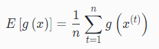
蒙特卡洛积分方法一般的想法是使用样本近似估计复杂分布的期望。具体地,我们获得一系列样本x(t),t=1,...,N,这些样本从p(x)中独立获得。在这种情况下,我们可以使用有限样本的累加近似估计期望:
在上述过程中,我们用适当样本的求和来代替积分。一般来说,近似计算的精确度可以通过增加n来提高。另外需要注意的是,近似计算的精确度取决于样本之间的独立性。当样本相互关联的时候,有效样本的数量减少了,这是MCMC的存在的一个潜在的问题。
2.2 马尔科夫链
Markov链是一个随机过程,我们利用顺序过程从一个状态过渡到另一个状态。我们在状态x(1)开始Markov链,使用转移函数p(x(t)∣x(t−1))作为状态的转移矩阵,确定下一个状态x(2)。然后以x(2)作为开始状态使用同样的转移函数继续确定下一个状态,如此重复,得到一系列状态:
x(1)→x(2)→...→x(t)→...
这样一个状态序列就被称为马尔科夫链(Markov chain)。生成一个包含T个状态的马尔科夫链的过程如下:
步骤
设t=1
生成一个初始值u,并设x(t)=u
重复下列过程
t=t+1
从转移函数p(x(t)∣x(t−1))中采样一个新的值
设x(t)=u
直到t=T
在上述迭代过程中,马尔科夫链的状态t+1仅仅是根据上一个状态t产生的。因此,马尔科夫链向新的状态转移总是只依赖最后一个状态。这是MCMC中使用马尔科夫链的很重要的一个属性。
当初始化每个马尔科夫链的时候,马尔科夫链将会在状态空间中进行状态转移。如果我们开始一系列的马尔科夫链,每一个链赋予不同的开始状态,通过一系列的状态转移过程,最终每个链都将处于接近起始状态的某个状态,这个过程被称为“burn-in”。马尔科夫链的一个重要的性质是,链的起始状态经过足够次数的转换后最终的状态不会受初始状态的影响(假定满足马尔科夫链的某些条件),也就是说,马尔科夫链经过有限次的状态转移之后,最终能达到稳定的状态,被称为平稳分布,从其平稳分布中可以反映样本。当满足一定的条件时,无论从哪个状态开始,马尔科夫链最终都会到达一个确定的稳定状态。应用到MCMC中,它允许我们从一个分布中连续地采样,且序列的初始状态不会影响估计过程。
举例
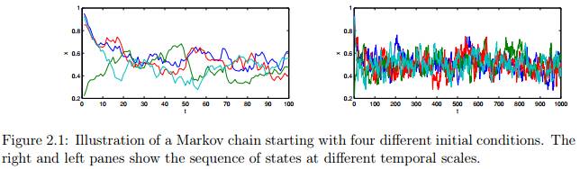
举个例子:图2.1展示了一个马尔科夫链的例子,为简单起见,以单个连续变量为例。从Beta分布中进行采样,分布函数为
Beta(200(0.9x(t−1)+0.05),200(1−0.9x(t−1)−0.05))。
从四个不同的起始状态开始,每个链都有T=1000次迭代。图中的两个子图分别展示了不同时刻的状态序列,线的颜色代表不同的链。注意,前10次迭代显示了序列对初始状态的依赖,这是“burn-in”过程。接下来序列的剩余部分是稳定状态(如果不停止,那么继续保持稳定状态)。那么我们如何确切知道稳定状态到达的时间,又怎么知道链是收敛的呢?要解释上述问题并不是容易的,尤其是在高维状态空间中。
2.3 综合讲解:马尔科夫链蒙特卡洛理论
前面两个部分讨论了MCMC理论背后的主要思想,蒙特卡洛采样和马尔科夫链。蒙特卡洛采样提供估计分布的各种特征:如均值,方差,峰值,或者其他的研究人员感兴趣的统计特征。马尔科夫链包含一个随机的顺序过程,并从平稳分布中采样状态。
MCMC的目标是设计一个马尔科夫链,该马尔科夫链的平稳分布就是我们要采样的分布,这就是所谓的目标分布。换句话说,我们希望从马尔科夫链的状态中采样等同于从目标分布中取样。这个想法是用一些方法设置转移函数,使无论马尔科夫链的初始状态是什么最终都能够收敛到目标分布。有很多方法使用相对简单的过程实现这个目标,我们在这里只讨论Metropolis,Metropolis Hastings和 Gibbs sampling。
2.4 Metropolis Sampling
Metropolis Sampling是最简单的MCMC方法,是Metropolis Hastings Sampling的一个特例,Metropolis Hastings Sampling将在下一节讨论。假设我们的目标是从目标密度函数p(θ)中采样,其中−∞<θ<∞。Metropolis sampler创建一个马尔科夫链并且产生一系列值:(注意由于公式编辑问题 θ(t) 和
θ(1)→θ(2)→...→θ(t)→...
其中θ(t)表示马尔科夫链在第t次迭代的状态。当“burn-in”过程之后,即达到平稳分布之后,从马尔科夫链中采样的样本反映了从目标分布p(θ)中的采样样本。
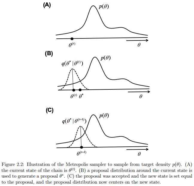
在Metropolis过程中,给第一个状态θ(1)初始化一些值。我们然后使用建议分布


为了决定是否接受该建议,我们定义一个偏差变量u,如果u≤α,我们接受这个建议,并将下一个状态设置为该建议:
步骤
设t=1
生成一个初始值,并设θ(t)=u
重复下列过程:
t=t+1
从q(θ∣θ(t−1))中生成一个建议θ∗
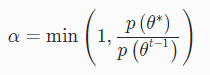
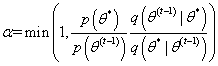
计算接受该建议的概率
从均匀分布Uniform(0,1)中生成一个值u
如果u≤α,接受该建议且设置θ(t)=θ∗;否则设置θ(t)=θ(t−1)
直到t=T
图2.2说明了两个状态序列转移的过程。为了直观地了解该过程为什么能从目标分布中获得样本,注意,如果新的建议分布得到的新状态的建议值相比旧节点状态更有可能在目标分布之下,公式(2.6)将始终接受新的建议。因此,采样器将移动到状态空间中,目标函数密度更高区域。然而,如果新的建议没有当前的状态好,仍然有可能接受这个“更糟糕”的建议并且转移到该建议状态。该过程总是接受“好的”建议,并且偶尔接受“坏的”建议,以确保采样器能探索整个状态空间,并且确保采样的样本从分布的所有部分获得(包含尾部)。
Metropolis sampler一个关键的要求是:建议分布是必须对称的,即: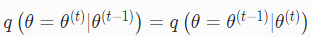
图 摘自LDA数学八卦,第31页
Metropolis sampler的主要优点是,公式(2.6)只包含了一个密度函数的比例。因此在函数p(θ)中任何独立于θ的项都可以被忽略。因此,我们不需要知道密度函数的归一化常量。并且该采样规则允许从非标准分布中采样,这是非常重要的,因为非标准分布在贝叶斯模型中经常用到。
举例
举个例子:假设我们希望从柯西分布中随机采样,给出柯西分布的概率密度如下面公式(2.7):
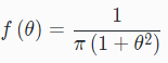
如何使用Metropolis sampler来模拟这个分布了,采样得到符合这个分布的样本?
答:
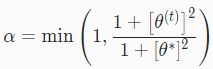
因为在Metropolis sampler过程中我们不需要标准化常量,所以将上式重写为公式2.8,:

因此,Metropolis接受概率变为:
我们使用正态分布作为建议分布,即从Normal(θ(t),σ)分布中产生建议。因此该分布的均值集中在当前状态,参数σ表示标准差需要人为设定,以控制建议分布的可变性。Listing 2.1展示了MATLAB函数,该函数返回非标准的柯西分布的密度。Listing 2.2展示了MATLAB代码实现的Metropolis sampler工具。图2.3展示了单个链经过500次迭代的模拟结果。其中,图2.3的第一个图展示了虚红线的理论密度,直方图展示了500个样本的分布。第二个图展示了样本的一个链。代码很简单,大家可以看看,不懂的可以在评论下方一起讨论。
1 function y = cauchy( theta ) 2 %% Returns the unnormalized density of the Cauchy distribution 3 y = 1 ./ (1 + theta.ˆ2);
Listing 2.1: Matlab function to evaluate the unnormalized Cauchy.
1 %% Chapter 2. Use Metropolis procedure to sample from Cauchy density 2 3 %% Initialize the Metropolis sampler 4 T = 500; % Set the maximum number of iterations 5 sigma = 1; % Set standard deviation of normal proposal density 6 thetamin = −30; thetamax = 30; % define a range for starting values 7 theta = zeros( 1 , T ); % Init storage space for our samples 8 seed=1; rand( 'state' , seed ); randn('state',seed ); % set the random seed 9 theta(1) = unifrnd( thetamin , thetamax ); % Generate start value 10 11 %% Start sampling 12 t = 1; 13 while t < T % Iterate until we have T samples 14 t = t + 1; 15 % Propose a new value for theta using a normal proposal density 16 theta star = normrnd( theta(t−1) , sigma ); 17 % Calculate the acceptance ratio 18 alpha = min( [ 1 cauchy( theta star ) / cauchy( theta(t−1) ) ] ); 19 % Draw a uniform deviate from [ 0 1 ] 20 u = rand; 21 % Do we accept this proposal? 22 if u < alpha 23 theta(t) = theta star; % If so, proposal becomes new state 24 else 25 theta(t) = theta(t−1); % If not, copy old state 26 end 27 end 28 29 %% Display histogram of our samples 30 figure( 1 ); clf; 31 subplot( 3,1,1 ); 32 nbins = 200; 33 thetabins = linspace( thetamin , thetamax , nbins ); 34 counts = hist( theta , thetabins ); 35 bar( thetabins , counts/sum(counts) , 'k' ); 36 xlim( [ thetamin thetamax ] ); 37 xlabel( '\theta' ); ylabel( 'p(\theta)' ); 38 39 %% Overlay the theoretical density 40 y = cauchy( thetabins ); 41 hold on; 42 plot( thetabins , y/sum(y) , 'r−−' , 'LineWidth' , 3 ); 43 set( gca , 'YTick' , [] ); 44 45 %% Display history of our samples 46 subplot( 3,1,2:3 ); 47 stairs( theta , 1:T , 'k−' ); 48 ylabel( 't' ); xlabel( '\theta' ); 49 set( gca , 'YDir' , 'reverse' ); 50 xlim( [ thetamin thetamax ] );
Listing 2.2: Matlab code to implement Metropolis sampler for Example 1

2.5 Metropolis-Hastings Sampling
Metropolis-Hasting (MH) sampler是Metropolis sampler的广义版本,我们既可以用对称的分布也可以用不对称的分布作为建议分布。MH sampler的工作方式与Metropolis sampler完全相同,但是使用下列公式计算接受概率:
上式中,MH sampler增加了一个额外的比例公式
MH sampler的过程如下:
步骤
设t=1
生成一个初始值u,并设θ(t)=u
重复下列过程:
t=t+1
从q(θ∣θ(t−1))中生成一个建议

计算接受该建议的概率
从均匀分布Uniform(0,1)中生成一个值u
如果u≤α,接受该建议且设置
;否则设置
 ;否则设置
;否则设置
直到t=T
实际上,不对称建议分布可以在Metropolis Hastings过程中使用,用以从目标分布中采样,这种采样方法也是有限制的。对于一个有界变量,应该在构造合适的建议分布的时候加以考虑。一般地,好的方法是针对目标分布选择具有良好密度函数的建议分布。例如,如果目标分布满足0≤θ≤∞,建议分布也应该满足此条件。
2.6 对多变量分布的Metropolis-Hastings
到目前为止,我们讨论的所有的例子都是基于单变量分布的。将MH sampler扩展到多变量分布是非常简单的。有两种不同的方法将采样过程从单个随机变量扩展到多变量空间中。
2.6.1 块更新(Blockwise updating)
第一种方法被称为Blockwise updating,我们使用一个与目标分布相同维度的建议分布。例如,我们想要从一个包含N个变量的概率分布中采样,我们就设计一个N维的建议分布,将建议分布(其中也包含N个变量)作为一个整体,要么接受要么拒绝。接下来,我们使用向量

步骤
设t=1
生成一个初始值
,并设
重复下列过程:
 ,并设
,并设
t=t+1
从
中生成一个建议
 中生成一个建议
计算接受该建议的概率
从均匀分布Uniform(0,1)中生成一个值u
如果u≤α,接受该建议且设置
;否则设置
 ;否则设置
;否则设置
直到 t=T
举例
示例1(adopted from Gill, 2008):假设我们想从二元变量空间指数分布中采样:

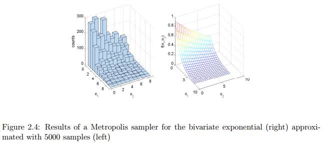
我们把其中的参数θ1和θ2的范围设置为[0,8],并且将其他参数设置如下:λ1=0.5,λ2=0.1,λ+0.01,max(θ1,θ2)=8。该二元分布的密度如图2.4(右图)所示。该密度函数的MATLAB实现如Listing 2.3所示。为了解释blockwise MH sampler,我们使用均匀分布作为建议分布,
1 function y = bivexp( theta1 , theta2 ) 2 %% Returns the density of a bivariate exponential function 3 lambda1 = 0.5; % Set up some constants 4 lambda2 = 0.1; 5 lambda = 0.01; 6 maxval = 8; 7 y = exp( −(lambda1+lambda)*theta1−(lambda2+lambda)*theta2−lambda*maxval );
Listing 2.3: Matlab code to implement bivariate density for Example 1
1 %% Chapter 2. Metropolis procedure to sample from Bivariate Exponential 2 % Blockwise updating. Use a uniform proposal distribution 3 4 %% Initialize the Metropolis sampler 5 T = 5000; % Set the maximum number of iterations 6 thetamin = [ 0 0 ]; % define minimum for theta1 and theta2 7 thetamax = [ 8 8 ]; % define maximum for theta1 and theta2 8 seed=1; rand( 'state' , seed ); randn('state',seed ); % set the random seed 9 theta = zeros( 2 , T ); % Init storage space for our samples 10 theta(1,1) = unifrnd( thetamin(1) , thetamax(1) ); % Start value for theta1 11 theta(2,1) = unifrnd( thetamin(2) , thetamax(2) ); % Start value for theta2 12 13 %% Start sampling 14 t = 1; 15 while t < T % Iterate until we have T samples 16 t = t + 1; 17 % Propose a new value for theta 18 theta star = unifrnd( thetamin , thetamax ); 19 pratio = bivexp( theta star(1) , theta star(2) ) / ... 20 bivexp( theta(1,t−1) , theta(2,t−1) ); 21 alpha = min( [ 1 pratio ] ); % Calculate the acceptance ratio 22 u = rand; % Draw a uniform deviate from [ 0 1 ] 23 if u < alpha % Do we accept this proposal? 24 theta(:,t) = theta star; % proposal becomes new value for theta 25 else 26 theta(:,t) = theta(:,t−1); % copy old value of theta 27 end 28 end 29 30 %% Display histogram of our samples 31 figure( 1 ); clf; 32 subplot( 1,2,1 ); 33 nbins = 10; 34 thetabins1 = linspace( thetamin(1) , thetamax(1) , nbins ); 35 thetabins2 = linspace( thetamin(2) , thetamax(2) , nbins ); 36 hist3( theta' , 'Edges' , {thetabins1 thetabins2} ); 37 xlabel( '\theta 1' ); ylabel('\theta 2' ); zlabel( 'counts' ); 38 az = 61; el = 30; 39 view(az, el); 40 41 %% Plot the theoretical density 42 subplot(1,2,2); 43 nbins = 20; 44 thetabins1 = linspace( thetamin(1) , thetamax(1) , nbins ); 45 thetabins2 = linspace( thetamin(2) , thetamax(2) , nbins ); 46 [ theta1grid , theta2grid ] = meshgrid( thetabins1 , thetabins2 ); 47 ygrid = bivexp( theta1grid , theta2grid ); 48 mesh( theta1grid , theta2grid , ygrid ); 49 xlabel( '\theta 1' ); ylabel('\theta 2' ); 50 zlabel( 'f(\theta 1,\theta 2)' ); 51 view(az, el);
Listing 2.4: Blockwise Metropolis-Hastings sampler for bivariate exponential distribution
举例
示例2:许多研究者提出概率模型用于解决信息排序问题,排序与很多优先排序问题有关:政治候选人的排名,汽车品牌,冰淇淋口味等。例如,假设要求一个人记住美国历届总统的时间顺序。 Steyvers, Lee, Miller, 和 Hemmer (2009)发现通过简单的概率模型可以捕获这些人在“美国总统排序”问题上犯的很多的错误,如Mallows模型。为了解释Mallows模型,我们先给出一个简单的例子。假设我们先看到五位美国总统是:华盛顿,亚当斯,杰斐逊,麦迪逊和门罗。我们用一个矢量来表示这个真正的顺序
w=(1,2,3,4,5)=(Washington,Adams,Jefferson,Madison,Monroe)
Mallows模型建议需要记住的排序应该是与真正的顺序相似的排序结果,使非常相近的排序比不相似的排序更有可能。具体来说,根据Mallows模型:一个人记住的排序
在上式中,是两个顺序矢量之间的Kendall tau distance距离。测量该距离即计算从一个序列到与另一个序列对齐所需要的交换次数。例如,如果θ=(Adams,Washington,Jefferson,Madison,Monroe),则,因为需要进行一次交换来使两个矢量序列相同。类似的,如果θ=(Adams,Jefferson,Washington,Madison,Monroe),则d(θ,w)=2,因为需要经过两次交换才能使两个序列对齐。注意,在Kendall tau distance距离中,只有相邻的项可以交换。参数λ控制矢量序列与真实序列的距离是如何达到峰值的。因此,通过增加λ,模型更有可能使矢量序列达到正确的排序。
现在的问题是,给定真实序列w和缩放参数λ,如何根据Mallows模型生成序列。基于此,可以用很简单的方法实现Metropolis sampler。采样器从开始,其对应一次随机的序列。每次迭代时,通过对当前状态进行稍微的修改,得到建议的序列。这种修改可以通过多种方法实现,这里的想法是,通过对当前的序列的任意项进行交换(而不只是相邻的项)来生成建议分布。即,通过下列建议分布公式(2.13)生成建议:
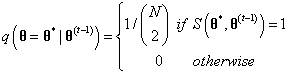
其中
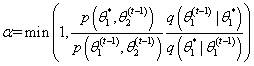
因为建议分布是对称的,所以我们可以使用Metropolis sampler,接受概率是公式(2.14):
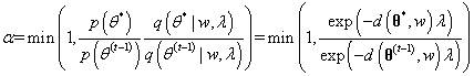
Kendall tau distance函数的MATLAB代码实现如Listing 2.5所示。Metropolis sampler的MATLAB代码实现如Listing 2.6所示。简单地展示了在总共500次迭代中每10次迭代的状态。下面是程序的一些示例输出:
1 function tau = kendalltau( order1 , order2 ) 2 %% Returns the Kendall tau distance between two orderings 3 % Note: this is not the most efficient implementation 4 [ dummy , ranking1 ] = sort( order1(:)' , 2 , 'ascend' ); 5 [ dummy , ranking2 ] = sort( order2(:)' , 2 , 'ascend' ); 6 N = length( ranking1 ); 7 [ ii , jj ] = meshgrid( 1:N , 1:N ); 8 ok = find( jj(:) > ii(:) ); 9 ii = ii( ok ); 10 jj = jj( ok ); 11 nok = length( ok ); 12 sign1 = ranking1( jj ) > ranking1( ii ); 13 sign2 = ranking2( jj ) > ranking2( ii ); 14 tau = sum( sign1 6= sign2 );
Listing 2.5: Function to evaluate Kendall tau distance
1 %% Chapter 2. Metropolis sampler for Mallows model 2 % samples orderings from a distribution over orderings 3 4 %% Initialize model parameters 5 lambda = 0.1; % scaling parameter 6 labels = { 'Washington' , 'Adams' , 'Jefferson' , 'Madison' , 'Monroe' }; 7 omega = [ 1 2 3 4 5 ]; % correct ordering 8 L = length( omega ); % number of items in ordering 9 10 %% Initialize the Metropolis sampler 11 T = 500; % Set the maximum number of iterations 12 seed=1; rand( 'state' , seed ); randn('state',seed ); % set the random seed 13 theta = zeros( L , T ); % Init storage space for our samples 14 theta(:,1) = randperm( L ); % Random ordering to start with 15 16 %% Start sampling 17 t = 1; 18 while t < T % Iterate until we have T samples 19 t = t + 1; 20 21 % Our proposal is the last ordering but with two items switched 22 lasttheta = theta(:,t−1); % Get the last theta 23 % Propose two items to switch 24 whswap = randperm( L ); whswap = whswap(1:2); 25 theta star = lasttheta; 26 theta star( whswap(1)) = lasttheta( whswap(2)); 27 theta star( whswap(2)) = lasttheta( whswap(1)); 28 29 % calculate Kendall tau distances 30 dist1 = kendalltau( theta star , omega ); 31 dist2 = kendalltau( lasttheta , omega ); 32 33 % Calculate the acceptance ratio 34 pratio = exp( −dist1*lambda ) / exp( −dist2*lambda ); 35 alpha = min( [ 1 pratio ] ); 36 u = rand; % Draw a uniform deviate from [ 0 1 ] 37 if u < alpha % Do we accept this proposal? 38 theta(:,t) = theta star; % proposal becomes new theta 39 else 40 theta(:,t) = lasttheta; % copy old theta 41 end 42 % Occasionally print the current state 43 if mod( t,10 ) == 0 44 fprintf( 't=%3d\t' , t ); 45 for j=1:L 46 fprintf( '%15s' , labels{ theta(j,t)} ); 47 end 48 fprintf( '\n' ); 49 end 50 end
Listing 2.6: Implementation of Metropolis-Hastings sampler for Mallows model
t=400 Jefferson Madison Adams Monroe Washington t=410 Washington Monroe Madison Jefferson Adams t=420 Washington Jefferson Madison Adams Monroe t=430 Jefferson Monroe Washington Adams Madison t=440 Washington Madison Monroe Adams Jefferson t=450 Jefferson Washington Adams Madison Monroe t=460 Washington Jefferson Adams Madison Monroe t=470 Monroe Washington Jefferson Adams Madison t=480 Adams Washington Monroe Jefferson Madison t=490 Adams Madison Jefferson Monroe Washington t=500 Monroe Adams Madison Jefferson Washington
2.6.2 Componentwise updating(单变量分别更新)
在blockwise updating更新中存在一个潜在的问题是,可能很难找到一个合适的高纬度建议分布。一个相关的问题是,blockwise updating可以被认为有高的拒绝率。接受或拒绝建议值
举例
例如,假定我们有一个二元分布θ=(θ1,θ2)。首先用合适的值初始化采样器的


步骤
设 t=1
生成一个初始值
,并设
重复下列过程:
 ,并设
,并设
t=1
从
中生成一个建议值
 中生成一个建议值
计算接受该建议的概率
从均匀分布Uniform(0,1)中生成一个值u
如果u≤α,接受该建议并令
,否则令
 ,否则令
,否则令
从
中生成一个建议
 中生成一个建议
计算接受该建议的概率
从均匀分布Uniform(0,1)中生成一个值u
如果u≤α,接受该建议并令
,否则令
 ,否则令
,否则令
直到 t=T
举例
示例3:我们从多元正态分布中采样,来说明componentwise sampler。首先设置多元正态分布的参数μ和Σ。参数μ是一个1×N的向量,参数Σ是一个N×N的协方差矩阵。在本例子中,我们使用二元正态分布,其中μ=(0,0)和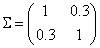
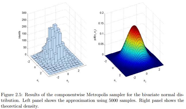
1 %% Chapter 2. Metropolis procedure to sample from Bivariate Normal 2 % Component−wise updating. Use a normal proposal distribution 3 4 %% Parameters of the Bivariate normal 5 mu = [ 0 0 ]; 6 sigma = [ 1 0.3; ... 7 0.3 1 ]; 8 9 %% Initialize the Metropolis sampler 10 T = 5000; % Set the maximum number of iterations 11 propsigma = 1; % standard dev. of proposal distribution 12 thetamin = [ −3 −3 ]; % define minimum for theta1 and theta2 13 thetamax = [ 3 3 ]; % define maximum for theta1 and theta2 14 seed=1; rand( 'state' , seed ); randn('state',seed ); % set the random seed 15 state = zeros( 2 , T ); % Init storage space for the state of the sampler 16 theta1 = unifrnd( thetamin(1) , thetamax(1) ); % Start value for theta1 17 theta2 = unifrnd( thetamin(2) , thetamax(2) ); % Start value for theta2 18 t = 1; % initialize iteration at 1 19 state(1,t) = theta1; % save the current state 20 state(2,t) = theta2; 21 22 %% Start sampling 23 while t < T % Iterate until we have T samples 24 t = t + 1; 25 26 %% Propose a new value for theta1 27 new theta1 = normrnd( theta1 , propsigma ); 28 pratio = mvnpdf( [ new theta1 theta2 ] , mu , sigma ) / ... 29 mvnpdf( [ theta1 theta2 ] , mu , sigma ); 30 alpha = min( [ 1 pratio ] ); % Calculate the acceptance ratio 31 u = rand; % Draw a uniform deviate from [ 0 1 ] 32 if u < alpha % Do we accept this proposal? 33 theta1 = new theta1; % proposal becomes new value for theta1 34 end 35 36 %% Propose a new value for theta2 37 new theta2 = normrnd( theta2 , propsigma ); 38 pratio = mvnpdf( [ theta1 new theta2 ] , mu , sigma ) / ... 39 mvnpdf( [ theta1 theta2 ] , mu , sigma ); 40 alpha = min( [ 1 pratio ] ); % Calculate the acceptance ratio 41 u = rand; % Draw a uniform deviate from [ 0 1 ] 42 if u < alpha % Do we accept this proposal? 43 theta2 = new theta2; % proposal becomes new value for theta2 44 end 45 46 %% Save state 47 state(1,t) = theta1; 48 state(2,t) = theta2; 49 end 50 51 %% Display histogram of our samples 52 figure( 1 ); clf; 53 subplot( 1,2,1 ); 54 nbins = 12; 55 thetabins1 = linspace( thetamin(1) , thetamax(1) , nbins ); 56 thetabins2 = linspace( thetamin(2) , thetamax(2) , nbins ); 57 hist3( state' , 'Edges' , {thetabins1 thetabins2} ); 58 xlabel( '\theta 1' ); ylabel('\theta 2' ); zlabel( 'counts' ); 59 az = 61; el = 30; view(az, el); 60 61 %% Plot the theoretical density 62 subplot(1,2,2); 63 nbins = 50; 64 thetabins1 = linspace( thetamin(1) , thetamax(1) , nbins ); 65 thetabins2 = linspace( thetamin(2) , thetamax(2) , nbins ); 66 [ theta1grid , theta2grid ] = meshgrid( thetabins1 , thetabins2 ); 67 zgrid = mvnpdf( [ theta1grid(:) theta2grid(:)] , mu , sigma ); 68 zgrid = reshape( zgrid , nbins , nbins ); 69 surf( theta1grid , theta2grid , zgrid ); 70 xlabel( '\theta 1' ); ylabel('\theta 2' ); 71 zlabel( 'pdf(\theta 1,\theta 2)' ); 72 view(az, el); 73 xlim([thetamin(1) thetamax(1)]); ylim([thetamin(2) thetamax(2)]);
Listing 2.7: Implementation of componentwise Metropolis sampler for bivariate normal
2.7 吉布斯采样(Gibbs Sampling)
Metropolis-Hastings和拒绝采样器的很大的缺点是其很难对于不同的建议分布调参(如何选取最好的建议分布),另外,该方法的一个好处是被拒绝的样本没有用于近似计算中。Gibbs sampler与这些不一样的是:方法采样得到所有的样本都被接受,从而提高了计算效率。另外一个优点是,研究人员不需要指定一个建议分布,这在MCMC过程中留下一些猜想。
然而,Gibbs sampler只能用于我们熟知的情况下,其特点是需要知道所有变量的联合概率分布,比如在多元分布中,我们必须知道每一个变量的联合条件分布,在某些情况下,这些条件分布是未知的,这时就不能使用Gibbs sampling。然而在很多贝叶斯模型中,都可以用Gibbs sampling对多元分布进行采样。
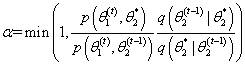
为了解释Gibbs sampler,我们以二元分布的情况为例,其联合分布是f(θ1,θ2)。Gibbs sampler所需要的关键条件是两个条件分布


步骤
设 t=1
生成一个初始值
,并设
重复下列过程:
 ,并设
,并设t=t+1
从条件分布
中采样
 中采样
中采样
从条件分布
中采样
 中采样
中采样
直到 t=T
举例
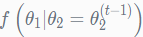
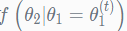
示例1:在上一章的“示例3”中,我们利用Metropolis sampler从二元正态分布中采样。二元正态分布也可以用Gibbs sampling进行高效的采样。在二元正态分布中设
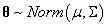
其中包括均值向量和协方差矩阵。本例子中,我们假设协方差矩阵是:

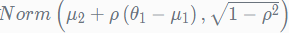
利用解析方法,我们推导出中
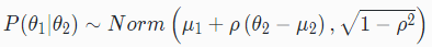
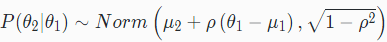
所以,Gibbs sampling的过程如下:
步骤
设 t=1
生成一个初始值
,并设
重复下列过程:
t=t+1
从条件分布
中采样
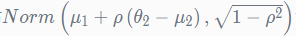

从条件分布
中采样

直到 t=T
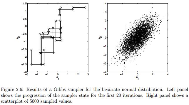
图2.6展示了利用Gibbs sampling二元正态分布的模拟结果,其中和。采样器共在一条链进行5000次迭代。右图展示了所有样本的散点图,左图模拟了前20次迭代的状态的进展。
到目前为止,MCMC这部分的内容翻译完毕,有些名词或者语句由于时间原因有问题,请大家随时提出来,谢谢了。
代码链接: http://pan.baidu.com/s/1qXIWzJu
MCMC matlab tutorial 电子版本:http://pan.baidu.com/s/1i48vyr7
Reference
Mark Steyver. Computational Statistics with Matlab. 2011
欢迎大家使用专知!点击阅读原文即可访问,访问专知,搜索主题-蒙特卡洛,获取更多关于马尔科夫链蒙特卡洛方法信息。
上面就是关于机器学习中马尔科夫链蒙特卡洛理论的一个总结,建议大家多多体会分布如何使用MCMC进行模拟,有什么问题可以在我们的专知公众号平台(桌面端或手机端直接访问 www.zhuanzhi.ai,一站式的AI知识服务)上交流或者加我们的专知-人工智能交流群 426491390
同时请,关注我们的公众号,获取最新关于专知以及人工智能的资讯、技术、算法等内容。扫一扫下方关注我们的微信公众号。

查看更多专知主题链路知识:
专知主题链路知识推荐#6-机器学习中似懂非懂的马尔科夫链蒙特卡洛采样(MCMC)入门教程01
专知主题链路知识推荐#1——马尔科夫链蒙特卡洛采样(附代码)
专知主题链路知识推荐#3——主题模型LDA Gibbs Sampling采样讲解
专知主题链路知识推荐#4-机器学习中往往被忽视的贝叶斯参数估计方法