通俗易懂!使用Excel和TF实现Transformer

作者 | 石晓文
转载自小小挖掘机(ID:wAIsjwj)
本文旨在通过最通俗易懂的过程来详解Transformer的每个步骤!
假设我们在做一个从中文翻译到英文的过程,我们的词表很简单如下:
中文词表:[机、器、学、习] 英文词表[deep、machine、learning、chinese]
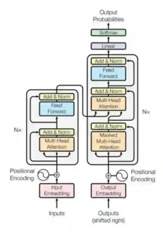
先来看一下Transformer的整个过程:
接下来,我们将按顺序来讲解Transformer的过程,并配有配套的excel计算过程和tensorflow代码。
先说明一下,本文的tensorflow代码中使用两条训练数据(因为实际场景中输入都是batch的),但excel计算只以第一条数据的处理过程为例。
1、Encoder输入
Encoder输入过程如下图所示:
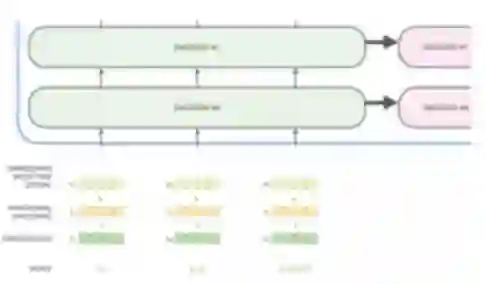
首先输入数据会转换为对应的embedding,然后会加上位置偏置,得到最终的输入。
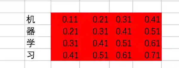
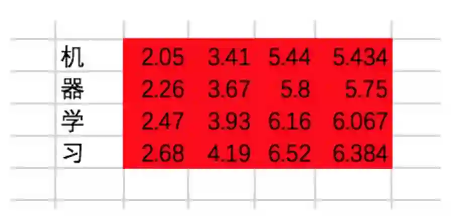
这里,为了结果的准确计算,我们使用常量来代表embedding,假设中文词表对应的embedding值分别是:
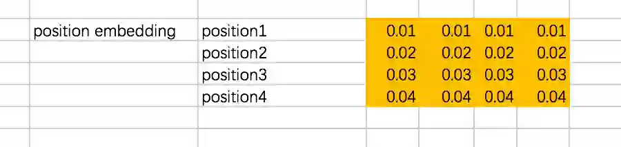
位置偏置position embedding使用下面的式子计算得出,注意这里位置偏置是包含两个维度的,不仅仅是encoder的第几个输入,同时embedding中的每一个维度都会加入位置偏置信息:
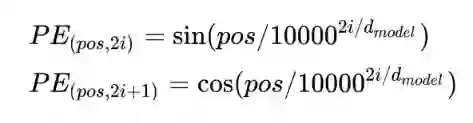
不过为了计算方便,我们仍然使用固定值代替:
假设我们有两条训练数据(Excel大都只以第一条数据为例):
[机、器、学、习] -> [ machine、learning]
[学、习、机、器] -> [learning、machine]
encoder的输入在转换成id后变为[[0,1,2,3],[2,3,0,1]]。
接下来,通过查找中文的embedding表,转换为embedding为:
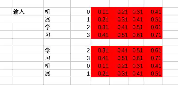
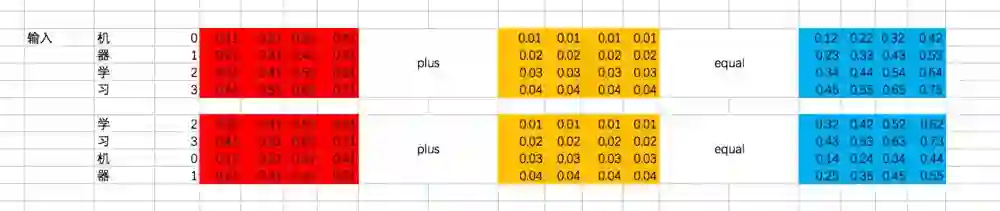
对输入加入位置偏置,注意这里是两个向量的对位相加:
上面的过程是这样的,接下来咱们用代码来表示一下:
import tensorflow as tf

chinese_embedding = tf.constant([[0.11,0.21,0.31,0.41],
                         [0.21,0.31,0.41,0.51],
                         [0.31,0.41,0.51,0.61],
                         [0.41,0.51,0.61,0.71]],dtype=tf.float32)


english_embedding = tf.constant([[0.51,0.61,0.71,0.81],
                         [0.52,0.62,0.72,0.82],
                         [0.53,0.63,0.73,0.83],
                         [0.54,0.64,0.74,0.84]],dtype=tf.float32)


position_encoding = tf.constant([[0.01,0.01,0.01,0.01],
                         [0.02,0.02,0.02,0.02],
                         [0.03,0.03,0.03,0.03],
                         [0.04,0.04,0.04,0.04]],dtype=tf.float32)

encoder_input = tf.constant([[0,1,2,3],[2,3,0,1]],dtype=tf.int32)


with tf.variable_scope("encoder_input"):
    encoder_embedding_input = tf.nn.embedding_lookup(chinese_embedding,encoder_input)
    encoder_embedding_input = encoder_embedding_input + position_encoding


with tf.Session() as sess:
    sess.run(tf.global_variables_initializer())
    print(sess.run([encoder_embedding_input]))
结果为:
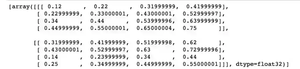
跟刚才的结果保持一致。
2、Encoder Block
一个Encoder的Block过程如下:
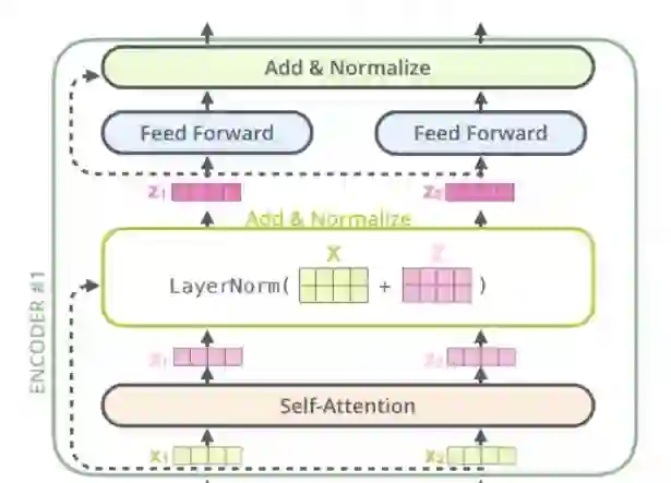
分为4步,分别是multi-head self attention、Add & Normalize、Feed Forward Network、Add & Normalize。
咱们主要来讲multi-head self attention。在讲multi-head self attention的时候,先讲讲Scaled Dot-Product Attention,我有时候也称为single-head self attention。
2.1 Attention机制简单回顾
Attention其实就是计算一种相关程度,看下面的例子:
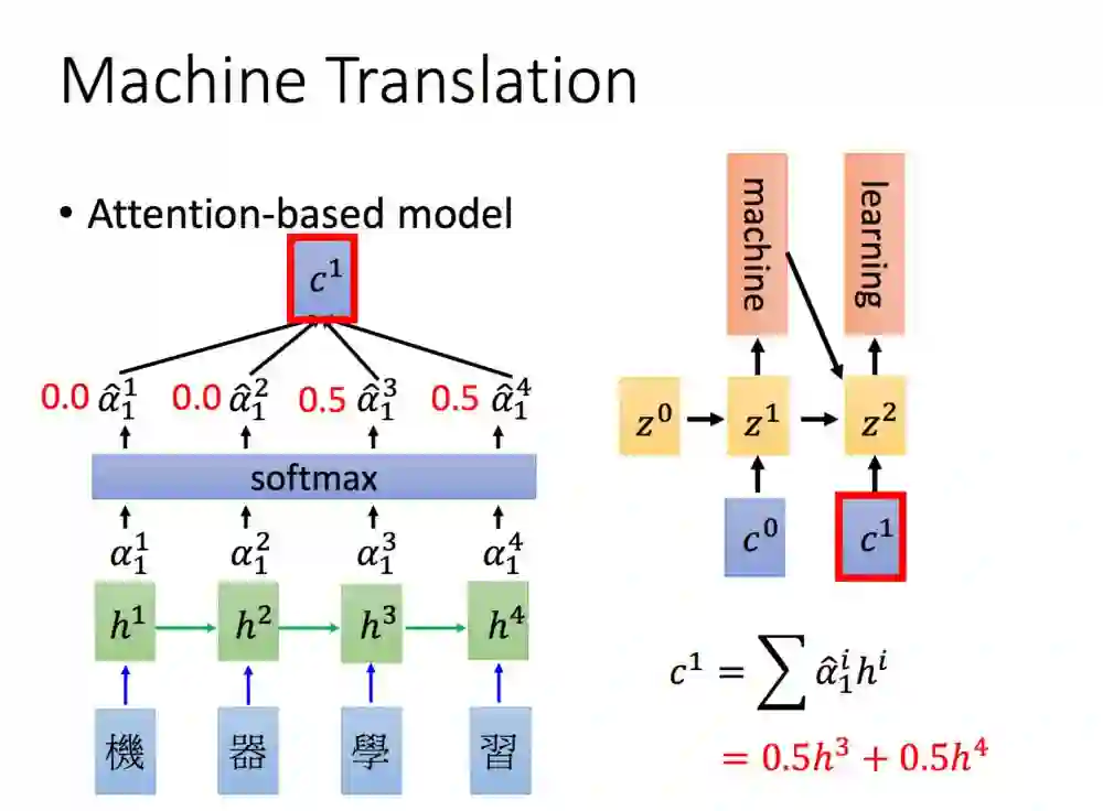
Attention通常可以进行如下描述,表示为将query(Q)和key-value pairs映射到输出上,其中query、每个key、每个value都是向量,输出是V中所有values的加权,其中权重是由Query和每个key计算出来的,计算方法分为三步:
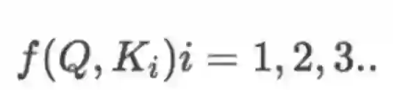
1)计算比较Q和K的相似度,用f来表示:
2)将得到的相似度进行softmax归一化:
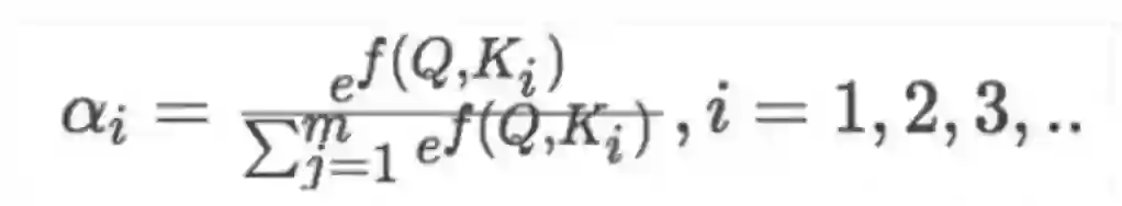
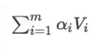
3)针对计算出来的权重,对所有的values进行加权求和,得到Attention向量:
计算相似度的方法有以下4种:
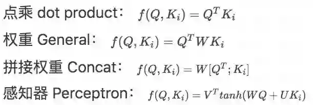
在本文中,我们计算相似度的方式是第一种。
2.2 Scaled Dot-Product Attention
咱们先说说Q、K、V。比如我们想要计算上图中machine和机、器、学、习四个字的attention,并加权得到一个输出,那么Query由machine对应的embedding计算得到,K和V分别由机、器、学、习四个字对应的embedding得到。
在encoder的self-attention中,由于是计算自身和自身的相似度,所以Q、K、V都是由输入的embedding得到的,不过我们还是加以区分。
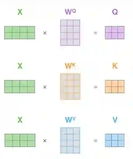
这里, Q、K、V分别通过一层全连接神经网络得到,同样,我们把对应的参数矩阵都写作常量。
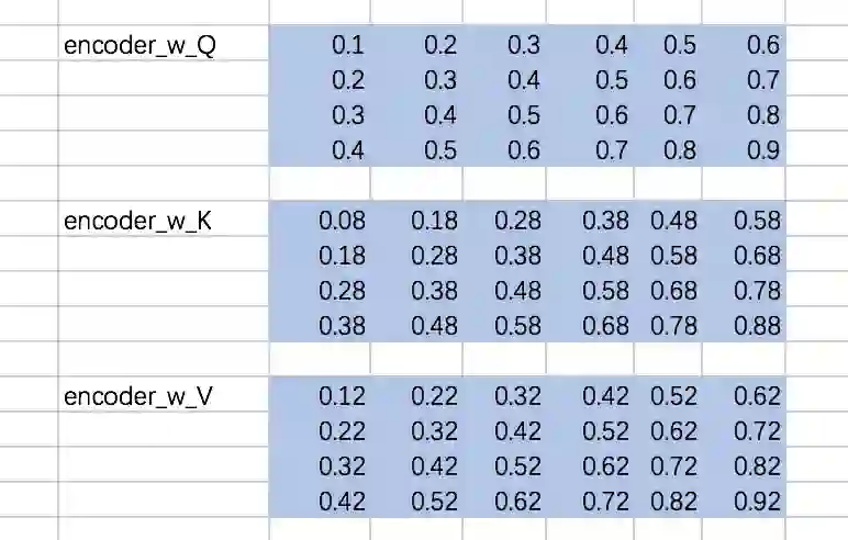
接下来,我们得到的到Q、K、V,我们以第一条输入为例:
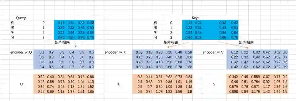
既然是一层全连接嘛,所以相当于一次矩阵相乘,excel里面的矩阵相乘如下:
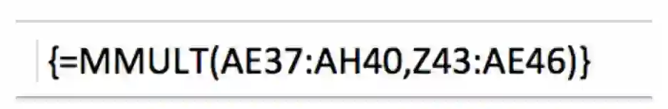
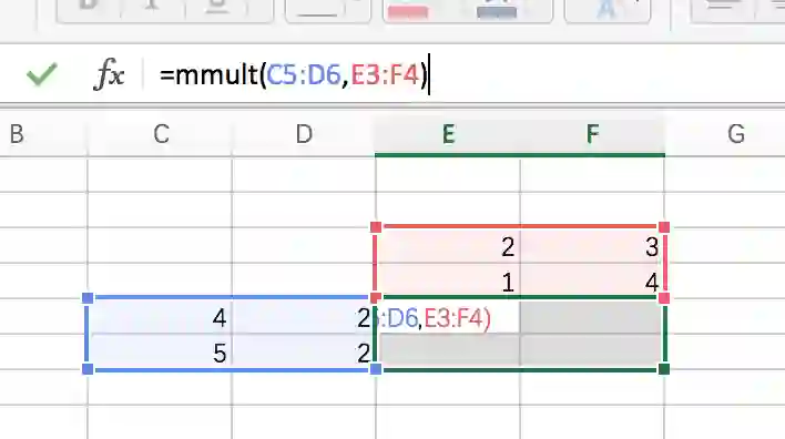
在Mac中,一定要先选中对应大小的区域,输入公式,然后使用command + shift + enter才能一次性得到全部的输出,如下图:
接下来,我们要去计算Q和K的相关性大小了,这里使用内积的方式,相当于QKT:
(上图应该是K,不影响整个过程理解)同样,excel中的转置,也要选择相应的区域后,使用transpose函数,然后按住command + shift + enter一次性得到全部输出。
我们来看看结果代表什么含义:
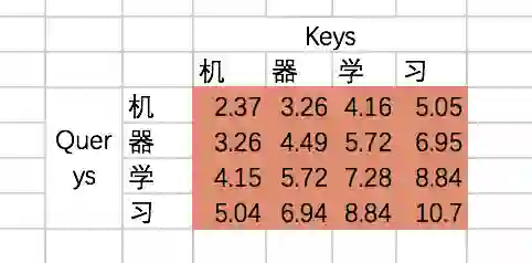
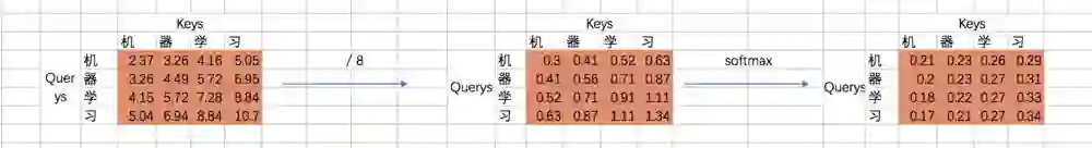
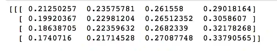
也就是说,机和机自身的相关性是2.37(未进行归一化处理),机和器的相关性是3.26,依次类推。我们可以称上述的结果为raw attention map。对于raw attention map,我们需要进行两步处理,首先是除以一个规范化因子,然后进行softmax操作,这里的规范化因子选择除以8,然后每行进行一个softmax归一化操作(按行做归一化是因为attention的初衷是计算每个Query和所有的Keys之间的相关性):
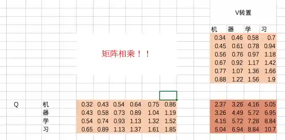
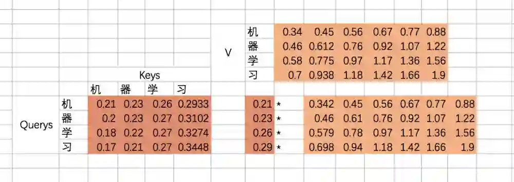
最后就是得到每个输入embedding 对应的输出embedding,也就是基于attention map对V进行加权求和,以“机”这个输入为例,最后的输出应该是V对应的四个向量的加权求和:
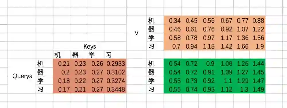
如果用矩阵表示,那么最终的结果是规范化后的attention map和V矩阵相乘,因此最终结果是:
至此,我们的Scaled Dot-Product Attention的过程就全部计算完了,来看看代码吧:
with tf.variable_scope("encoder_scaled_dot_product_attention"):
    encoder_Q = tf.matmul(tf.reshape(encoder_embedding_input,(-1,tf.shape(encoder_embedding_input)[2])),w_Q)
    encoder_K = tf.matmul(tf.reshape(encoder_embedding_input,(-1,tf.shape(encoder_embedding_input)[2])),w_K)
    encoder_V = tf.matmul(tf.reshape(encoder_embedding_input,(-1,tf.shape(encoder_embedding_input)[2])),w_V)

    encoder_Q = tf.reshape(encoder_Q,(tf.shape(encoder_embedding_input)[0],tf.shape(encoder_embedding_input)[1],-1))
    encoder_K = tf.reshape(encoder_K,(tf.shape(encoder_embedding_input)[0],tf.shape(encoder_embedding_input)[1],-1))
    encoder_V = tf.reshape(encoder_V,(tf.shape(encoder_embedding_input)[0],tf.shape(encoder_embedding_input)[1],-1))


    attention_map = tf.matmul(encoder_Q,tf.transpose(encoder_K,[0,2,1]))
    attention_map = attention_map / 8
    attention_map = tf.nn.softmax(attention_map)


with tf.Session() as sess:
    sess.run(tf.global_variables_initializer())
    print(sess.run(attention_map))
    print(sess.run(encoder_first_sa_output))
第一条数据的attention map为:
第一条数据的输出为:
可以看到,跟我们通过excel计算得到的输出也是保持一致的。
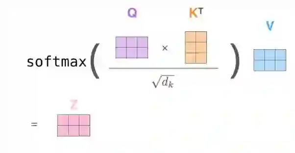
咱们再通过图片来回顾下Scaled Dot-Product Attention的过程:
2.3 multi-head self attention
Multi-Head Attention就是把Scaled Dot-Product Attention的过程做H次,然后把输出Z合起来。
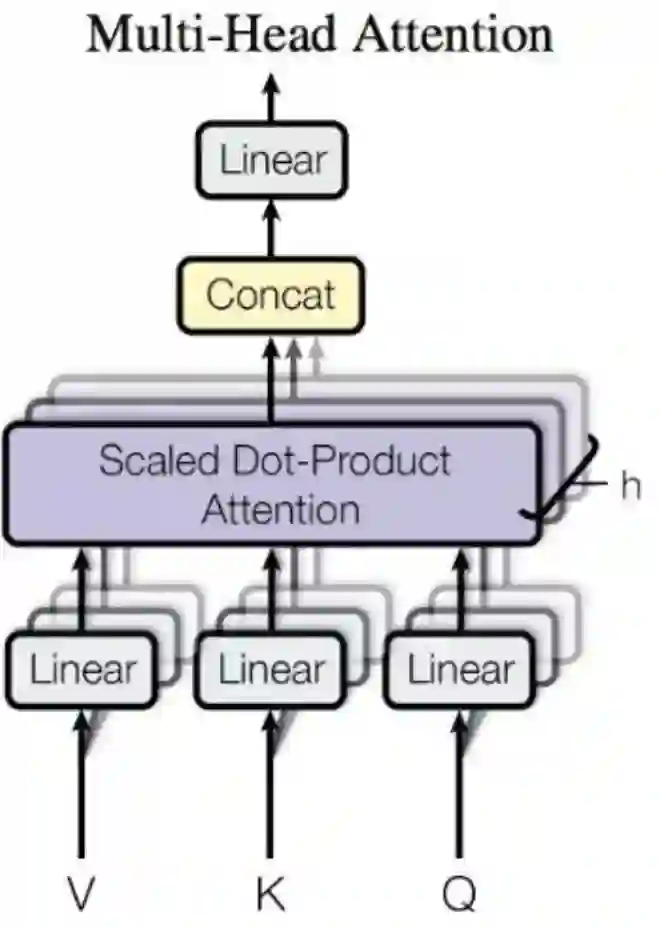
整个过程图示如下:
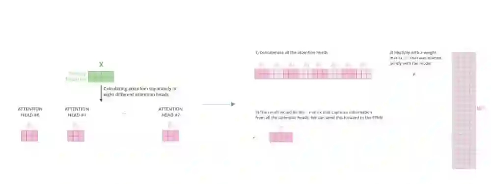
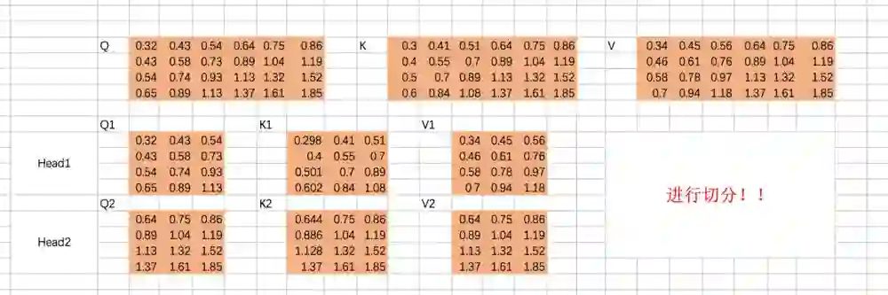
这里,我们还是先用excel的过程计算一遍。假设我们刚才计算得到的Q、K、V从中间切分,分别作为两个Head的输入:
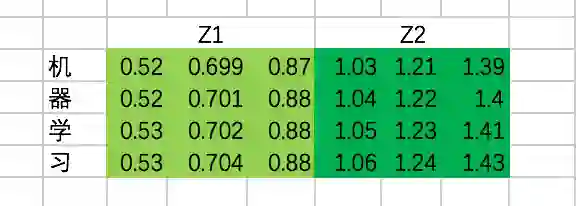
重复上面的Scaled Dot-Product Attention过程,我们分别得到两个Head的输出:
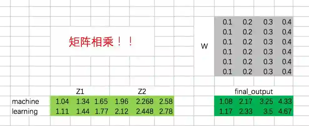
接下来,我们需要通过一个权重矩阵,来得到最终输出。
为了我们能够进行后面的Add的操作,我们需要把输出的长度和输入保持一致,即每个单词得到的输出embedding长度保持为4。
同样,我们这里把转换矩阵W设置为常数:
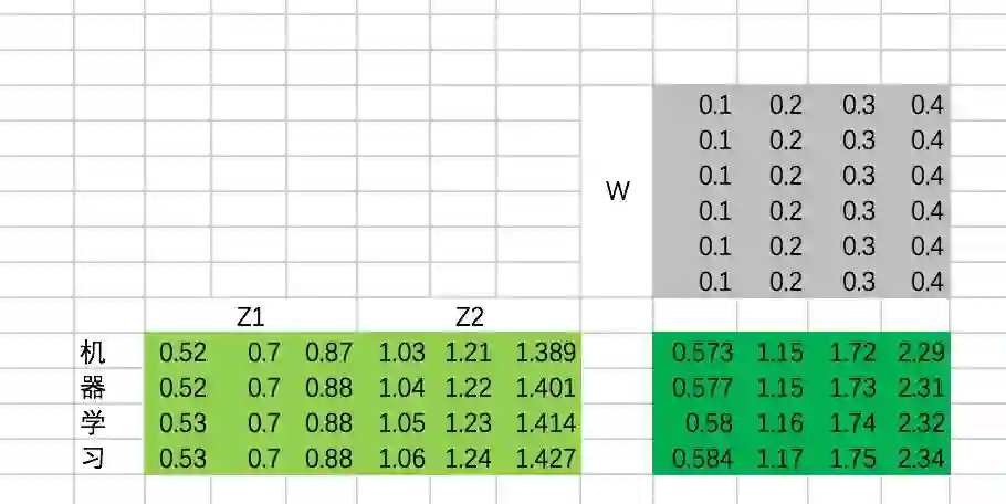
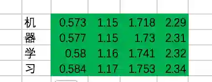
最终,每个单词在经过multi-head attention之后,得到的输出为:
好了,开始写代码吧:
w_Z = tf.constant([[0.1,0.2,0.3,0.4],
                   [0.1,0.2,0.3,0.4],
                   [0.1,0.2,0.3,0.4],
                   [0.1,0.2,0.3,0.4],
                   [0.1,0.2,0.3,0.4],
                   [0.1,0.2,0.3,0.4]],dtype=tf.float32)


with tf.variable_scope("encoder_input"):
    encoder_embedding_input = tf.nn.embedding_lookup(chinese_embedding,encoder_input)
    encoder_embedding_input = encoder_embedding_input + position_encoding

with tf.variable_scope("encoder_multi_head_product_attention"):
    encoder_Q = tf.matmul(tf.reshape(encoder_embedding_input,(-1,tf.shape(encoder_embedding_input)[2])),w_Q)
    encoder_K = tf.matmul(tf.reshape(encoder_embedding_input,(-1,tf.shape(encoder_embedding_input)[2])),w_K)
    encoder_V = tf.matmul(tf.reshape(encoder_embedding_input,(-1,tf.shape(encoder_embedding_input)[2])),w_V)

    encoder_Q = tf.reshape(encoder_Q,(tf.shape(encoder_embedding_input)[0],tf.shape(encoder_embedding_input)[1],-1))
    encoder_K = tf.reshape(encoder_K,(tf.shape(encoder_embedding_input)[0],tf.shape(encoder_embedding_input)[1],-1))
    encoder_V = tf.reshape(encoder_V,(tf.shape(encoder_embedding_input)[0],tf.shape(encoder_embedding_input)[1],-1))

    encoder_Q_split = tf.split(encoder_Q,2,axis=2)
    encoder_K_split = tf.split(encoder_K,2,axis=2)
    encoder_V_split = tf.split(encoder_V,2,axis=2)

    encoder_Q_concat = tf.concat(encoder_Q_split,axis=0)
    encoder_K_concat = tf.concat(encoder_K_split,axis=0)
    encoder_V_concat = tf.concat(encoder_V_split,axis=0)

    attention_map = tf.matmul(encoder_Q_concat,tf.transpose(encoder_K_concat,[0,2,1]))
    attention_map = attention_map / 8
    attention_map = tf.nn.softmax(attention_map)

    weightedSumV = tf.matmul(attention_map,encoder_V_concat)

    outputs_z = tf.concat(tf.split(weightedSumV,2,axis=0),axis=2)

    outputs = tf.matmul(tf.reshape(outputs_z,(-1,tf.shape(outputs_z)[2])),w_Z)
    outputs = tf.reshape(outputs,(tf.shape(encoder_embedding_input)[0],tf.shape(encoder_embedding_input)[1],-1))

import numpy as np
with tf.Session() as sess:
#     print(sess.run(encoder_Q))
#     print(sess.run(encoder_Q_split))
    #print(sess.run(weightedSumV))
    #print(sess.run(outputs_z))
    print(sess.run(outputs))
结果的输出为:
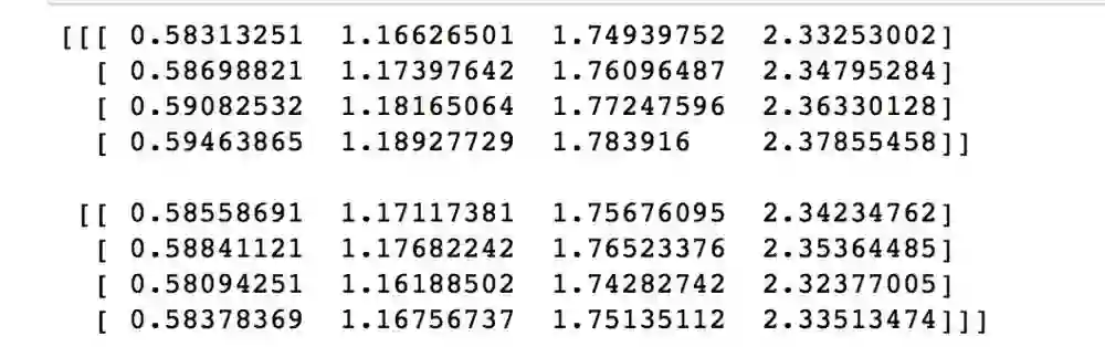
这里的结果其实和excel是一致的,细小的差异源于excel在复制粘贴过程中,小数点的精度有所损失。
这里我们主要来看下两个函数,分别是split和concat,理解这两个函数的过程对明白上述代码至关重要。
split函数主要有三个参数,第一个是要split的tensor,第二个是分割成几个tensor,第三个是在哪一维进行切分。也就是说, encoder_Q_split = tf.split(encoder_Q,2,axis=2),执行这段代码的话,encoder_Q这个tensor会按照axis=2切分成两个同样大的tensor,这两个tensor的axis=0和axis=1维度的长度是不变的,但axis=2的长度变为了一半,我们在后面通过图示的方式来解释。
从代码可以看到,共有两次split和concat的过程,第一次是将Q、K、V切分为不同的Head:
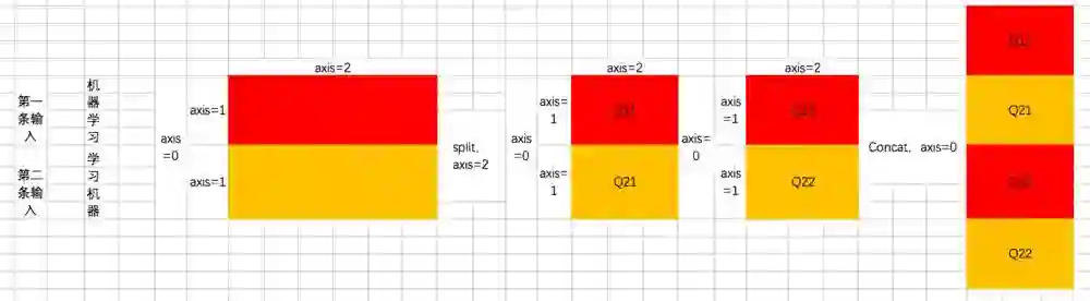
也就是说,原先每条数据的所对应的各Head的Q并非相连的,而是交替出现的,即 [Head1-Q11,Head1-Q21,Head2-Q12,Head2-Q22]
第二次是最后计算完每个Head的输出Z之后,通过split和concat进行还原,过程如下:
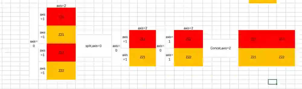
上面的图示咱们将三维矩阵操作抽象成了二维,我加入了axis的说明帮助你理解。如果不懂的话,单步执行下代码就会懂啦。
2.4 Add & Normalize & FFN
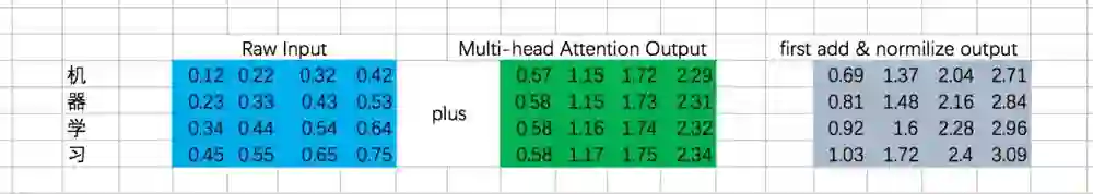
后面的过程其实很多简单了,我们继续用excel来表示一下,这里,我们忽略BN的操作(大家可以加上,这里主要是比较麻烦哈哈)
第一次Add & Normalize
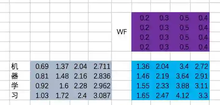
接下来是一个FFN,我们仍然假设是固定的参数,那么output是:
第二次Add & Normalize
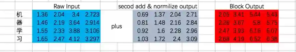
我们终于在经过一个Encoder的Block后得到了每个输入对应的输出,分别为:
让我们把这段代码补充上去吧:
with tf.variable_scope("encoder_block"):
    encoder_Q = tf.matmul(tf.reshape(encoder_embedding_input,(-1,tf.shape(encoder_embedding_input)[2])),w_Q)
    encoder_K = tf.matmul(tf.reshape(encoder_embedding_input,(-1,tf.shape(encoder_embedding_input)[2])),w_K)
    encoder_V = tf.matmul(tf.reshape(encoder_embedding_input,(-1,tf.shape(encoder_embedding_input)[2])),w_V)

    encoder_Q = tf.reshape(encoder_Q,(tf.shape(encoder_embedding_input)[0],tf.shape(encoder_embedding_input)[1],-1))
    encoder_K = tf.reshape(encoder_K,(tf.shape(encoder_embedding_input)[0],tf.shape(encoder_embedding_input)[1],-1))
    encoder_V = tf.reshape(encoder_V,(tf.shape(encoder_embedding_input)[0],tf.shape(encoder_embedding_input)[1],-1))

    encoder_Q_split = tf.split(encoder_Q,2,axis=2)
    encoder_K_split = tf.split(encoder_K,2,axis=2)
    encoder_V_split = tf.split(encoder_V,2,axis=2)

    encoder_Q_concat = tf.concat(encoder_Q_split,axis=0)
    encoder_K_concat = tf.concat(encoder_K_split,axis=0)
    encoder_V_concat = tf.concat(encoder_V_split,axis=0)

    attention_map = tf.matmul(encoder_Q_concat,tf.transpose(encoder_K_concat,[0,2,1]))
    attention_map = attention_map / 8
    attention_map = tf.nn.softmax(attention_map)

    weightedSumV = tf.matmul(attention_map,encoder_V_concat)

    outputs_z = tf.concat(tf.split(weightedSumV,2,axis=0),axis=2)

    sa_outputs = tf.matmul(tf.reshape(outputs_z,(-1,tf.shape(outputs_z)[2])),w_Z)
    sa_outputs = tf.reshape(sa_outputs,(tf.shape(encoder_embedding_input)[0],tf.shape(encoder_embedding_input)[1],-1))


    sa_outputs = sa_outputs + encoder_embedding_input

    # todo :add BN
    W_f = tf.constant([[0.2,0.3,0.5,0.4],
                       [0.2,0.3,0.5,0.4],
                       [0.2,0.3,0.5,0.4],
                       [0.2,0.3,0.5,0.4]])

    ffn_outputs = tf.matmul(tf.reshape(sa_outputs,(-1,tf.shape(sa_outputs)[2])),W_f)
    ffn_outputs = tf.reshape(ffn_outputs,(tf.shape(sa_outputs)[0],tf.shape(sa_outputs)[1],-1))

    encoder_outputs = ffn_outputs + sa_outputs
    # todo :add BN

import numpy as np
with tf.Session() as sess:
#     print(sess.run(encoder_Q))
#     print(sess.run(encoder_Q_split))
    #print(sess.run(weightedSumV))
    #print(sess.run(outputs_z))
    #print(sess.run(sa_outputs))
    #print(sess.run(ffn_outputs))
    print(sess.run(encoder_outputs))
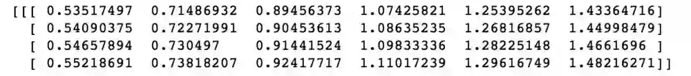
输出为:
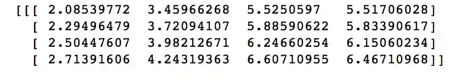
与excel计算结果基本一致。
当然,encoder的各层是可以堆叠的,但我们这里只以单层的为例,重点是理解整个过程。
3、Decoder Block
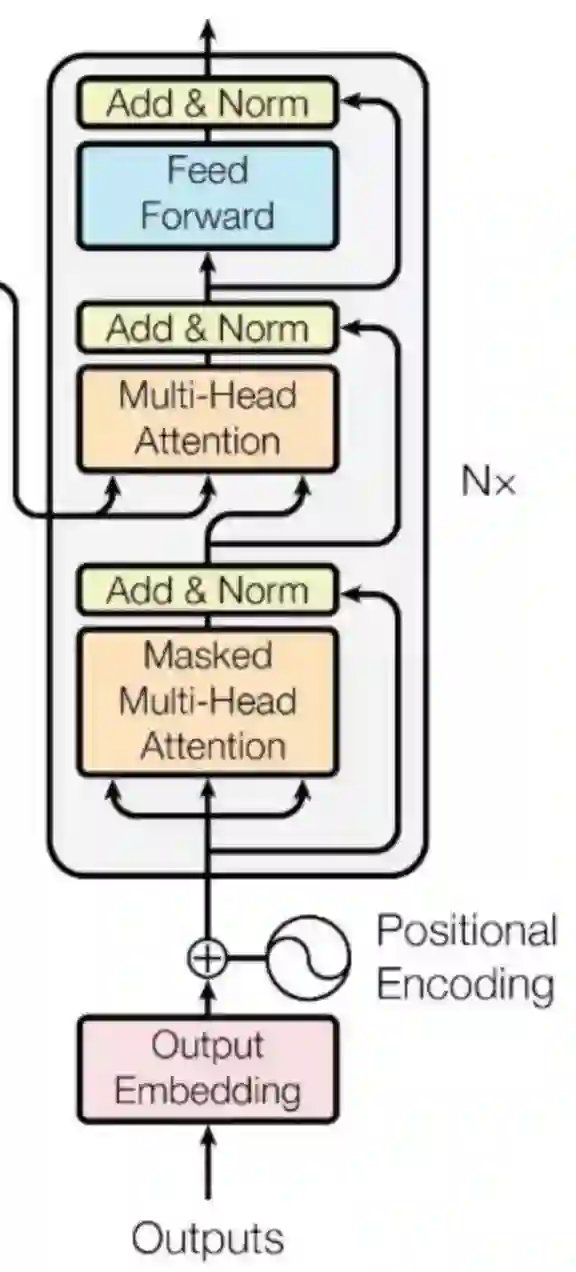
一个Decoder的Block过程如下:
相比Encoder,这里的过程分为6步,分别是 masked multi-head self attention、Add & Normalize、encoder-decoder attention、Add & Normalize、Feed Forward Network、Add & Normalize。
咱们还是重点来讲masked multi-head self attention和encoder-decoder attention。
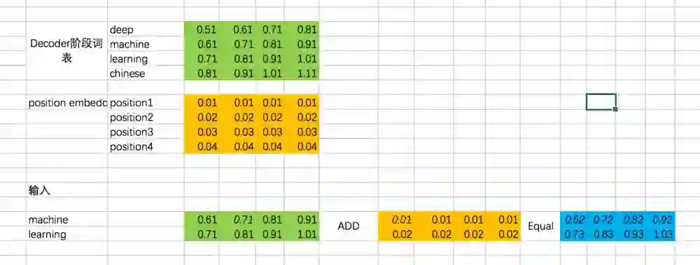
3.1 Decoder输入
这里,在excel中,咱们还是以第一条输入为例,来展示整个过程:
[机、器、学、习] -> [ machine、learning]
因此,Decoder阶段的输入是:
对应的代码如下:
english_embedding = tf.constant([[0.51,0.61,0.71,0.81],
                         [0.61,0.71,0.81,0.91],
                         [0.71,0.81,0.91,1.01],
                         [0.81,0.91,1.01,1.11]],dtype=tf.float32)


position_encoding = tf.constant([[0.01,0.01,0.01,0.01],
                         [0.02,0.02,0.02,0.02],
                         [0.03,0.03,0.03,0.03],
                         [0.04,0.04,0.04,0.04]],dtype=tf.float32)

decoder_input = tf.constant([[1,2],[2,1]],dtype=tf.int32)

with tf.variable_scope("decoder_input"):
    decoder_embedding_input = tf.nn.embedding_lookup(english_embedding,decoder_input)
    decoder_embedding_input = decoder_embedding_input + position_encoding[0:tf.shape(decoder_embedding_input)[1]]
3.2 masked multi-head self attention
这个过程和multi-head self attention基本一致,只不过对于decoder来说,得到每个阶段的输出时,我们是看不到后面的信息的。举个例子,我们的第一条输入是:[机、器、学、习] -> [ machine、learning] ,decoder阶段两次的输入分别是machine和learning,在输入machine时,我们是看不到learning的信息的,因此在计算attention的权重的时候,machine和learning的权重是没有的。我们还是先通过excel来演示一下,再通过代码来理解:
计算Attention的权重矩阵是:
仍然以两个Head为例,计算Q、K、V:
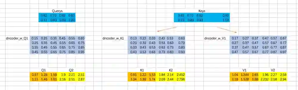
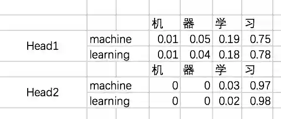
分别计算两个Head的attention map
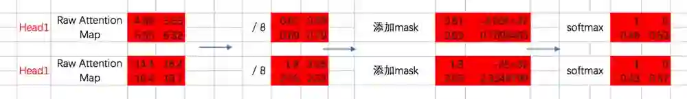
咱们先来实现这部分的代码,masked attention map的计算过程:
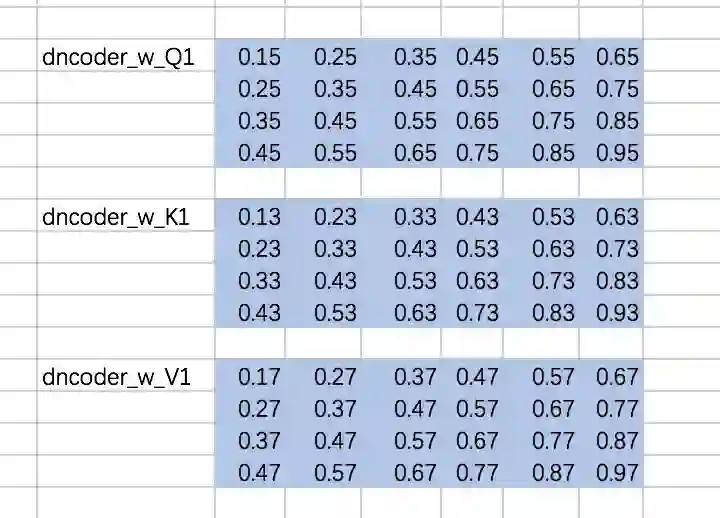
先定义下权重矩阵,同encoder一样,定义成常数:
w_Q_decoder_sa = tf.constant([[0.15,0.25,0.35,0.45,0.55,0.65],
                   [0.25,0.35,0.45,0.55,0.65,0.75],
                   [0.35,0.45,0.55,0.65,0.75,0.85],
                   [0.45,0.55,0.65,0.75,0.85,0.95]],dtype=tf.float32)

w_K_decoder_sa = tf.constant([[0.13,0.23,0.33,0.43,0.53,0.63],
                   [0.23,0.33,0.43,0.53,0.63,0.73],
                   [0.33,0.43,0.53,0.63,0.73,0.83],
                   [0.43,0.53,0.63,0.73,0.83,0.93]],dtype=tf.float32)

w_V_decoder_sa = tf.constant([[0.17,0.27,0.37,0.47,0.57,0.67],
                   [0.27,0.37,0.47,0.57,0.67,0.77],
                   [0.37,0.47,0.57,0.67,0.77,0.87],
                   [0.47,0.57,0.67,0.77,0.87,0.97]],dtype=tf.float32)
随后,计算添加mask之前的attention map:
with tf.variable_scope("decoder_sa_block"):
    decoder_Q = tf.matmul(tf.reshape(decoder_embedding_input,(-1,tf.shape(decoder_embedding_input)[2])),w_Q_decoder_sa)
    decoder_K = tf.matmul(tf.reshape(decoder_embedding_input,(-1,tf.shape(decoder_embedding_input)[2])),w_K_decoder_sa)
    decoder_V = tf.matmul(tf.reshape(decoder_embedding_input,(-1,tf.shape(decoder_embedding_input)[2])),w_V_decoder_sa)

    decoder_Q = tf.reshape(decoder_Q,(tf.shape(decoder_embedding_input)[0],tf.shape(decoder_embedding_input)[1],-1))
    decoder_K = tf.reshape(decoder_K,(tf.shape(decoder_embedding_input)[0],tf.shape(decoder_embedding_input)[1],-1))
    decoder_V = tf.reshape(decoder_V,(tf.shape(decoder_embedding_input)[0],tf.shape(decoder_embedding_input)[1],-1))

    decoder_Q_split = tf.split(decoder_Q,2,axis=2)
    decoder_K_split = tf.split(decoder_K,2,axis=2)
    decoder_V_split = tf.split(decoder_V,2,axis=2)

    decoder_Q_concat = tf.concat(decoder_Q_split,axis=0)
    decoder_K_concat = tf.concat(decoder_K_split,axis=0)
    decoder_V_concat = tf.concat(decoder_V_split,axis=0)

    decoder_sa_attention_map_raw = tf.matmul(decoder_Q_concat,tf.transpose(decoder_K_concat,[0,2,1]))
    decoder_sa_attention_map = decoder_sa_attention_map_raw / 8
随后,对attention map添加mask:
diag_vals = tf.ones_like(decoder_sa_attention_map[0,:,:])
tril = tf.contrib.linalg.LinearOperatorTriL(diag_vals).to_dense()
masks = tf.tile(tf.expand_dims(tril,0),[tf.shape(decoder_sa_attention_map)[0],1,1])
paddings = tf.ones_like(masks) * (-2 ** 32 + 1)
decoder_sa_attention_map = tf.where(tf.equal(masks,0),paddings,decoder_sa_attention_map)
decoder_sa_attention_map = tf.nn.softmax(decoder_sa_attention_map)
这里我们首先构造一个全1的矩阵diag_vals,这个矩阵的大小同attention map。随后通过tf.contrib.linalg.LinearOperatorTriL方法把上三角部分变为0,该函数的示意如下:
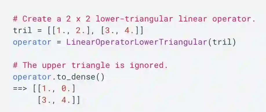
基于这个函数生成的矩阵tril,我们便可以构造对应的mask了。不过需要注意的是,对于我们要加mask的地方,不能赋值为0,而是需要赋值一个很小的数,这里为-2^32 + 1。因为我们后面要做softmax,e^0=1,是一个很大的数啦。
运行上面的代码:
import numpy as np
with tf.Session() as sess:
    print(sess.run(decoder_sa_attention_map))
观察第一条数据对应的结果如下:
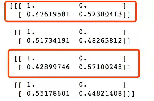
与我们excel计算结果相吻合。
后面的过程我们就不详细介绍了,我们直接给出经过masked multi-head self attention的对应结果:
对应的代码如下:
weightedSumV = tf.matmul(decoder_sa_attention_map,decoder_V_concat)

decoder_outputs_z = tf.concat(tf.split(weightedSumV,2,axis=0),axis=2)

decoder_sa_outputs = tf.matmul(tf.reshape(decoder_outputs_z,(-1,tf.shape(decoder_outputs_z)[2])),w_Z_decoder_sa)

decoder_sa_outputs = tf.reshape(decoder_sa_outputs,(tf.shape(decoder_embedding_input)[0],tf.shape(decoder_embedding_input)[1],-1))


with tf.Session() as sess:
    print(sess.run(decoder_sa_outputs))
输出为:

与excel保持一致!
3.3 encoder-decoder attention
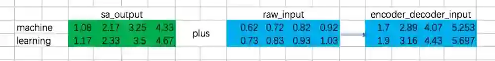
在encoder-decoder attention之间,还有一个Add & Normalize的过程,同样,我们忽略 Normalize,只做Add操作:
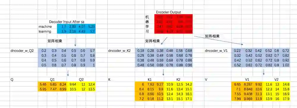
接下来,就是encoder-decoder了,这里跟multi-head attention相同,但是需要注意的一点是,我们这里想要做的是,计算decoder的每个阶段的输入和encoder阶段所有输出的attention,所以Q的计算通过decoder对应的embedding计算,而K和V通过encoder阶段输出的embedding来计算:
接下来,计算Attention Map,注意,这里attention map的大小为2 * 4的,每一行代表一个decoder的输入,与所有encoder输出之间的attention score。同时,我们不需要添加mask,因为decoder的输入是可以看到所有encoder的输出信息的。得到的attention map结果如下:
哈哈,这里数是我瞎写的,结果不太好,不过不影响对整个过程的理解。
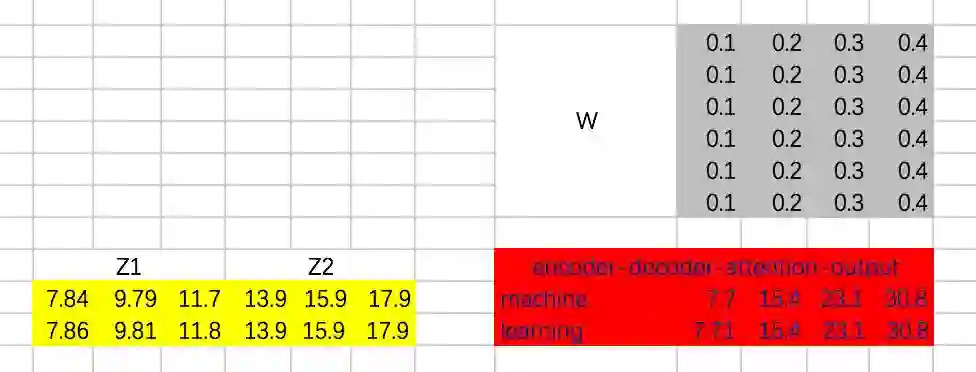
接下来,我们得到整个encoder-decoder阶段的输出为:
接下来,还有Add & Normalize、Feed Forward Network、Add & Normalize过程,咱们这里就省略了。直接上代码吧:
w_Q_decoder_sa2 = tf.constant([[0.2,0.3,0.4,0.5,0.6,0.7],
                   [0.3,0.4,0.5,0.6,0.7,0.8],
                   [0.4,0.5,0.6,0.7,0.8,0.9],
                   [0.5,0.6,0.7,0.8,0.9,1]],dtype=tf.float32)

w_K_decoder_sa2 = tf.constant([[0.18,0.28,0.38,0.48,0.58,0.68],
                   [0.28,0.38,0.48,0.58,0.68,0.78],
                   [0.38,0.48,0.58,0.68,0.78,0.88],
                   [0.48,0.58,0.68,0.78,0.88,0.98]],dtype=tf.float32)

w_V_decoder_sa2 = tf.constant([[0.22,0.32,0.42,0.52,0.62,0.72],
                   [0.32,0.42,0.52,0.62,0.72,0.82],
                   [0.42,0.52,0.62,0.72,0.82,0.92],
                   [0.52,0.62,0.72,0.82,0.92,1.02]],dtype=tf.float32)

w_Z_decoder_sa2 = tf.constant([[0.1,0.2,0.3,0.4],
                   [0.1,0.2,0.3,0.4],
                   [0.1,0.2,0.3,0.4],
                   [0.1,0.2,0.3,0.4],
                   [0.1,0.2,0.3,0.4],
                   [0.1,0.2,0.3,0.4]],dtype=tf.float32)


with tf.variable_scope("decoder_encoder_attention_block"):

    decoder_sa_outputs = decoder_sa_outputs + decoder_embedding_input

    encoder_decoder_Q = tf.matmul(tf.reshape(decoder_sa_outputs,(-1,tf.shape(decoder_sa_outputs)[2])),w_Q_decoder_sa2)
    encoder_decoder_K = tf.matmul(tf.reshape(encoder_outputs,(-1,tf.shape(encoder_outputs)[2])),w_K_decoder_sa2)
    encoder_decoder_V = tf.matmul(tf.reshape(encoder_outputs,(-1,tf.shape(encoder_outputs)[2])),w_V_decoder_sa2)

    encoder_decoder_Q = tf.reshape(encoder_decoder_Q,(tf.shape(decoder_embedding_input)[0],tf.shape(decoder_embedding_input)[1],-1))
    encoder_decoder_K = tf.reshape(encoder_decoder_K,(tf.shape(encoder_outputs)[0],tf.shape(encoder_outputs)[1],-1))
    encoder_decoder_V = tf.reshape(encoder_decoder_V,(tf.shape(encoder_outputs)[0],tf.shape(encoder_outputs)[1],-1))

    encoder_decoder_Q_split = tf.split(encoder_decoder_Q,2,axis=2)
    encoder_decoder_K_split = tf.split(encoder_decoder_K,2,axis=2)
    encoder_decoder_V_split = tf.split(encoder_decoder_V,2,axis=2)

    encoder_decoder_Q_concat = tf.concat(encoder_decoder_Q_split,axis=0)
    encoder_decoder_K_concat = tf.concat(encoder_decoder_K_split,axis=0)
    encoder_decoder_V_concat = tf.concat(encoder_decoder_V_split,axis=0)

    encoder_decoder_attention_map_raw = tf.matmul(encoder_decoder_Q_concat,tf.transpose(encoder_decoder_K_concat,[0,2,1]))
    encoder_decoder_attention_map = encoder_decoder_attention_map_raw / 8

    encoder_decoder_attention_map = tf.nn.softmax(encoder_decoder_attention_map)

    weightedSumV = tf.matmul(encoder_decoder_attention_map,encoder_decoder_V_concat)

    encoder_decoder_outputs_z = tf.concat(tf.split(weightedSumV,2,axis=0),axis=2)

    encoder_decoder_outputs = tf.matmul(tf.reshape(encoder_decoder_outputs_z,(-1,tf.shape(encoder_decoder_outputs_z)[2])),w_Z_decoder_sa2)

    encoder_decoder_attention_outputs = tf.reshape(encoder_decoder_outputs,(tf.shape(decoder_embedding_input)[0],tf.shape(decoder_embedding_input)[1],-1))

    encoder_decoder_attention_outputs = encoder_decoder_attention_outputs + decoder_sa_outputs

    # todo :add BN
    W_f = tf.constant([[0.2,0.3,0.5,0.4],
                       [0.2,0.3,0.5,0.4],
                       [0.2,0.3,0.5,0.4],
                       [0.2,0.3,0.5,0.4]])

    decoder_ffn_outputs = tf.matmul(tf.reshape(encoder_decoder_attention_outputs,(-1,tf.shape(encoder_decoder_attention_outputs)[2])),W_f)
    decoder_ffn_outputs = tf.reshape(decoder_ffn_outputs,(tf.shape(encoder_decoder_attention_outputs)[0],tf.shape(encoder_decoder_attention_outputs)[1],-1))

    decoder_outputs = decoder_ffn_outputs + encoder_decoder_attention_outputs
    # todo :add BN

with tf.Session() as sess:
    print(sess.run(decoder_outputs))
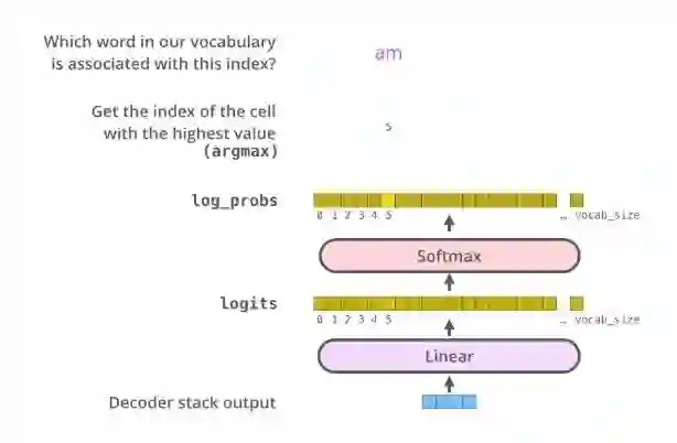
4、全连接层及最终输出
最后的全连接层很简单了,对于decoder阶段的输出,通过全连接层和softmax之后,最终得到选择每个单词的概率,并计算交叉熵损失:
这里,我们直接给出代码:
W_final = tf.constant([[0.2,0.3,0.5,0.4],
                       [0.2,0.3,0.5,0.4],
                       [0.2,0.3,0.5,0.4],
                       [0.2,0.3,0.5,0.4]])

logits = tf.matmul(tf.reshape(decoder_outputs,(-1,tf.shape(decoder_outputs)[2])),W_final)
logits = tf.reshape(logits,(tf.shape(decoder_outputs)[0],tf.shape(decoder_outputs)[1],-1))


logits = tf.nn.softmax(logits)

y = tf.one_hot(decoder_input,depth=4)

loss = tf.nn.softmax_cross_entropy_with_logits(logits=logits,labels=y)

train_op = tf.train.AdamOptimizer(learning_rate=0.0001).minimize(loss)
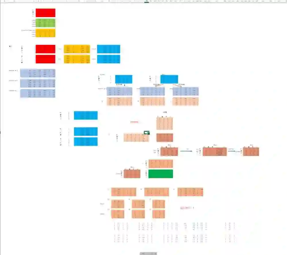
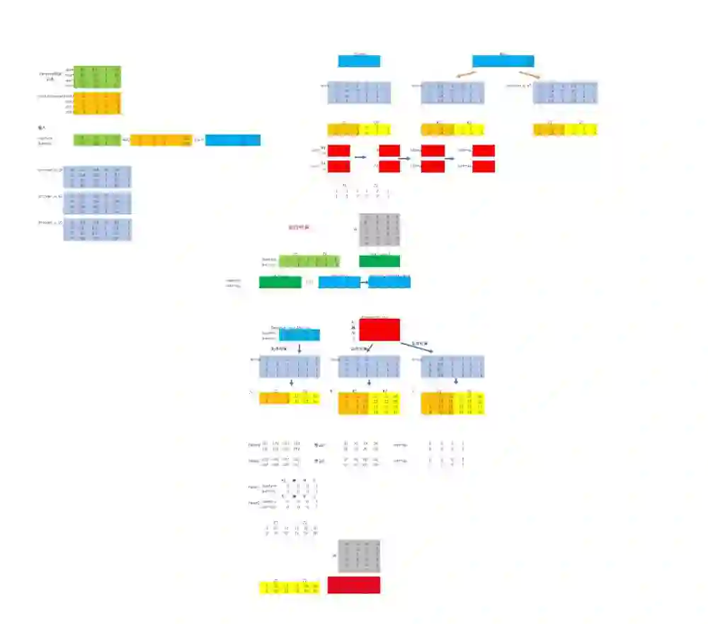
整个文章下来,咱们不仅通过excel实现了一遍transorform的正向传播过程,还通过tf代码实现了一遍。放两张excel的抽象图,就知道是多么浩大的工程了:
好了,文章最后,咱们再来回顾一下整个Transformer的结构:
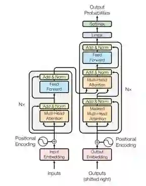
希望通过本文,你能够对Transformer的整体结构有个更清晰的认识!
(*本文为 AI科技大本营转载文章,转载请联系原作者)
◆
精彩推荐
◆
大会开幕倒计时8天!
2019以太坊技术及应用大会特邀以太坊创始人V神与众多海内外知名技术专家齐聚北京,聚焦区块链技术,把握时代机遇,深耕行业应用,共话以太坊2.0新生态。即刻扫码,享优惠票价。


推荐阅读