倾向得分加权匹配分析方法的R实现

声明：本文最早发表于公众号：每天进步一点点2015，已征得作者同意

1.1 PSW Package 简介

• PSW : Propensity Score Weighting Methods for Dichotomous Treatments.

      该包由Huzhang Mao 和LiangLi两位作者贡献，首次发布于2017年10月；该包主要运用倾向得分加权分析方法实现因果效应的推断；主要由5个函数模块构成：

（1）倾向得分共同取值范围以及各匹配变量的标准化偏差的可视化图示；

（2）检验匹配后数据是否平衡（平衡性假设检验）；

（3）倾向值模型设定检验；

（4）处理效应的加权估计；

（5）处理效应的双重稳健性估计；

      由于篇幅所限，本文仅关注对average treatment effect of the treated (ATT)的估计。

1.1.1 载入需要的程辑包

# 加载第三方包
# 为读入本文所需要用到的Stata数据集
library(haven) 
library(RStata)
library(readstata13)
library(foreign)
#同时载入需要的程辑包
library(stats)  
library(Hmisc)
library(survival)
library(Formula)
library(ggplot2)
library(gtools)
library(graphics)
library(lattice)
library(PSW)
# 读取ldw_exper.dta数据集ldw_exper <- read_dta(file = file.choose())
# 强制转换为数据框结构
ldwdf <- as.data.frame(ldw_exper) #转换为数据框格式，便于计算
# 变量激活，便于直接使用变量名
attach(ldwdf)

1.1.2 本文使用的数据集（ldw_exper.dta）简介

      该数据集介绍可参见《高级计量经济学与Stata应用第二版（陈强）》；
re78为1978年实际收入，t是否参加就业培训，age年龄，educ教育年限，black是否为黑人，hisp是否为拉丁族，married是否结婚，re74、re75为1974和75年的实际收入，u74，u75为74和75年是否为失业状态；笔者选择该数据集，核心目的对照书中传统的倾向得分匹配分析方法与本文所介绍的用倾向得分加权匹配分析方法的异同。

1.2 Propensity score weighting in R

本节主要介绍倾向得分加权匹配分析的实现过程.

1.2.1 构建 Propensity score model

# generate Propensity score model
form.ps <- "t ~ age + educ + black + hisp+married+re74+re75+u74+u75"
# calculate Standardized differnce with "ATT"
tmp1 <- psw( data = ldwdf, form.ps = form.ps, weight = "ATT" )
# display ps.model  
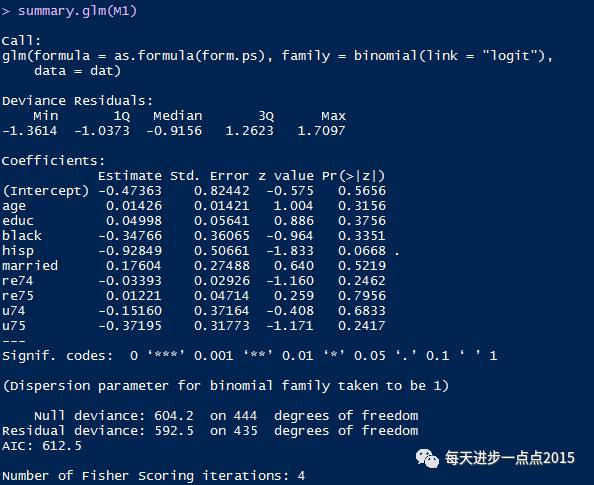
M1<-tmp1$ps.model
summary.glm(M1)
#由于glm函数未给出logit模型的整体性是否显著P值，故需通过手动编制计算
with(M1, pchisq(null.deviance - deviance, df.null - df.residual, lower.tail = FALSE))

结果输出：

1.2.2 平衡性检验 Balance checking using standardized mean difference

# generate A vector of covariates
V.name <- c("age","educ","black", "hisp","married","re74","re75","u74","u75")
#  compute the standardized mean difference for balance diagnosis.
tmp2 <- psw.balance( data = ldwdf, weight = "ATT", form.ps = form.ps,
V.name = V.name )
# 为方便演示，此处仅提取匹配前、后的标准化均值差异 
tmp2$std.diff.before;
tmp2$std.diff.after;

输出结果：

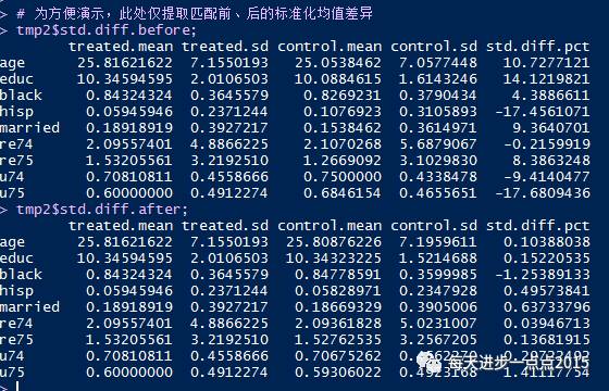
我们可以进一步提取以下非常有用的信息，具体包括以下内容（fitted propensity score model, estimated propenstity scores, estimated propensity score weights, standardized mean difference before and after weighting adjustment）.从tmp2列示的结果来看，我们发现，通过倾向得分加权法，匹配后偏差大幅度下降，通过了平衡性检验。

1.2.3 模型设定检验 Propensity score model specification test

      This test is a goodness-of-fit test of propensity score model. 备注:该检验原假设为倾向性得分模型被正确设定

# generate A vector of transformation types for covariates in V.name.
trans.type <- c( "identity","identity","identity","identity","identity","identity","identity","identity","identity") 
#  compute Propensity score model specification test.
tmp3<-psw.spec.test( data = ldwdf, weight = "ATT", form.ps = form.ps,
V.name = V.name, trans.type = trans.type )
#  为方便演示，这里仅提取 Propensity score model specification test的P值信息
tmp3$pvalue

      由此，我们可以得出模型设定不拒绝原假设，可以接受被正确设定的结论。

1.2.4 Propensity score weighting estimator

      This is used to estimate the weighted estimator, and make inference using the sandwich variance estimator that takes into account the sampling variability in the estimated propensity score.

备注:仍以估计ATT的值为例；需注意一下gaussian和binomial的用法

# estimate the weighted treatment effect estimator.
tmp4 <- psw.wt( data = ldwdf, weight = "ATT", form.ps = form.ps,
out.var = "re78", family = "binomial" )
# display tmp4
head(tmp4)

结果输出：

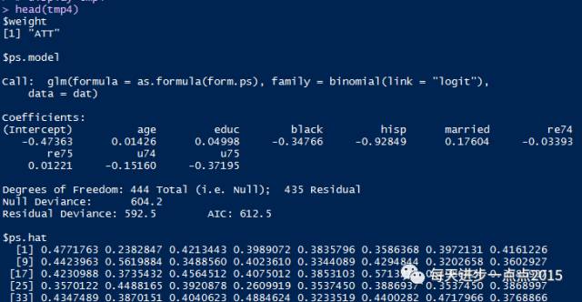
可以根据自己需求提取相应信息,包括本部分所关心的weighted estimator for risk difference、standard error for est.risk.wt、weighted estimator for relative risk以及standard error  for est.rr.wt等内容.

小结：

用倾向得分加权分析方法得到的ATT值为1.7381，标准误为0.6887，与传统的PSM分析所用的匹配方法得出的结论基本一致。

感谢：

非常感谢各位网友向“每天进步一点点2015”公众号投递原创性文章，同时也欢迎各位网友一起参与知识分享和交流。

欢迎大家关注微信公众号：数萃大数据

课程公告

深度学习培训班【上海站】

时间：2017年12月23-24日

地点：上海创梦云实训创新中心

更多详情，请扫描下面二维码