word2Vec总结

2019 年 11 月 2 日 AINLP

这是一篇比较早之前总结的文章，内容虽然简单，但是个人认为轻松易懂，Word2Vec 是自然语言处理技术的基石，深刻理解 Word2Vec 原理对 NLPlayer 至关重要。

一直以来，对，以及对里面的实现原因一直模糊不清，由此决心阅读的两篇原始论文，，，看完以后还是有点半懂半不懂的感觉，于是又结合网上的一些比较好的讲解（Word2Vec Tutorial - The Skip-Gram Model^[1])，以及开源的实现代码理解了一遍，在此总结一下。

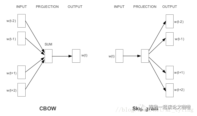
下面主要以模型来介绍。

word2vec 工作流程

只是一个三层的神经网络。
喂给模型一个，然后用来预测它周边的词。
然后去掉最后一层，只保存和。
从词表中选取一个词，喂给模型，在将会给出该词的。

import numpy as np
import tensorflow as tf
corpus_raw = 'He is the king . The king is royal . She is the royal  queen '
# convert to lower case
corpus_raw = corpus_raw.lower()

上述代码非常简单和易懂，现在我们需要获取，假设我们现在有这样一个任务，喂给模型一个词，我们需要获取它周边的词，举例来说，就是获取该词前个和后个词，那么这个就是代码中的，例如下图：

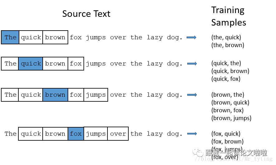
注意：如果这个词是一个句子的开头或结尾，忽略窗外的词。

我们需要对文本数据进行一个简单的预处理，创建一个的字典和的字典。

words = []
for word in corpus_raw.split():
    if word != '.': # because we don't want to treat . as a word
        words.append(word)
words = set(words) # so that all duplicate words are removed
word2int = {}
int2word = {}
vocab_size = len(words) # gives the total number of unique words
for i,word in enumerate(words):
    word2int[word] = i
    int2word[i] = word

来看看这个字典有啥效果：

print(word2int['queen'])
-> 42 (say)
print(int2word[42])
-> 'queen'

好，现在可以获取训练数据啦

data = []
WINDOW_SIZE = 2
for sentence in sentences:
    for word_index, word in enumerate(sentence):
        for nb_word in sentence[max(word_index - WINDOW_SIZE, 0) : min(word_index + WINDOW_SIZE, len(sentence)) + 1] :
            if nb_word != word:
                data.append([word, nb_word])

上述代码就是切句子，然后切词，得出的一个个训练样本，其中就是模型输入，就是该词周边的某个单词。

把打印出来看看？

print(data)
[['he', 'is'],
 ['he', 'the'],
 ['is', 'he'],
 ['is', 'the'],
 ['is', 'king'],
 ['the', 'he'],
 ['the', 'is'],
 ['the', 'king'],
.
.
.
]

现在我们有了训练数据了，但是需要将它转成模型可读可理解的形式，这时，上面的字典的作用就来了。

来，我们更进一步的对进行处理，并使其转成向量

i.e.,
say we have a vocabulary of 3 words : pen, pineapple, apple
where
word2int['pen'] -> 0 -> [1 0 0]
word2int['pineapple'] -> 1 -> [0 1 0]
word2int['apple'] -> 2 -> [0 0 1]

那么为啥是特征呢？稍后将解释。

# function to convert numbers to one hot vectors
def to_one_hot(data_point_index, vocab_size):
    temp = np.zeros(vocab_size)
    temp[data_point_index] = 1
    return temp
x_train = [] # input word
y_train = [] # output word
for data_word in data:
    x_train.append(to_one_hot(word2int[ data_word[0] ], vocab_size))
    y_train.append(to_one_hot(word2int[ data_word[1] ], vocab_size))
# convert them to numpy arrays
x_train = np.asarray(x_train)
y_train = np.asarray(y_train)

利用建立模型

# making placeholders for x_train and y_train
x = tf.placeholder(tf.float32, shape=(None, vocab_size))
y_label = tf.placeholder(tf.float32, shape=(None, vocab_size))

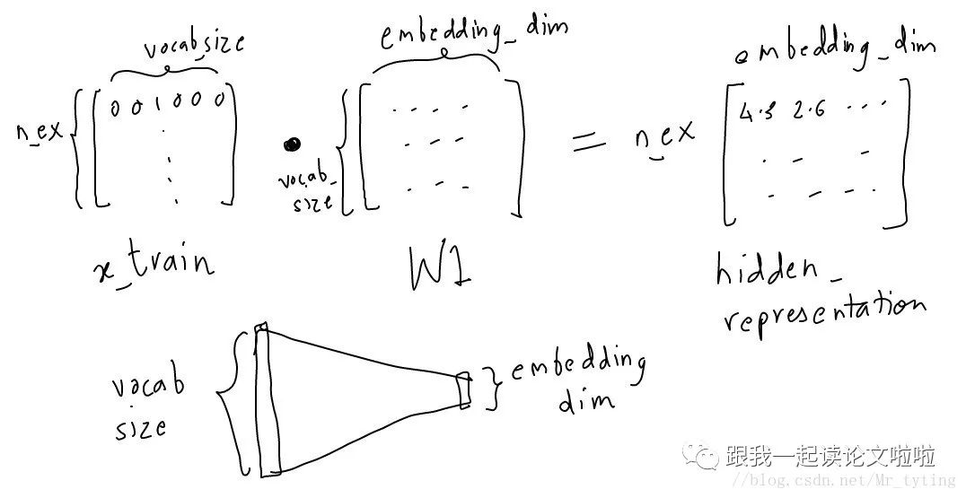
由上图，我们可以看出，我们将转换成，并且将维度降低到设定的。

EMBEDDING_DIM = 5 # you can choose your own number
W1 = tf.Variable(tf.random_normal([vocab_size, EMBEDDING_DIM]))
b1 = tf.Variable(tf.random_normal([EMBEDDING_DIM])) #bias
hidden_representation = tf.add(tf.matmul(x,W1), b1)

接下来，我们需要使用函数来预测该周边的词。

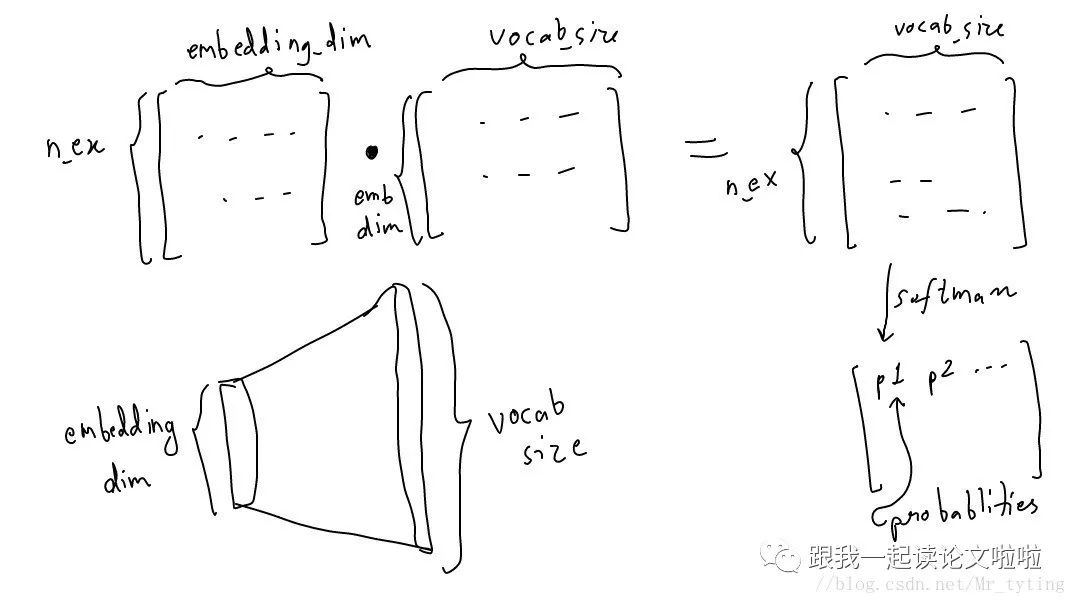
W2 = tf.Variable(tf.random_normal([EMBEDDING_DIM, vocab_size]))
b2 = tf.Variable(tf.random_normal([vocab_size]))
prediction = tf.nn.softmax(tf.add( tf.matmul(hidden_representation, W2), b2))

所以整体的过程如下：

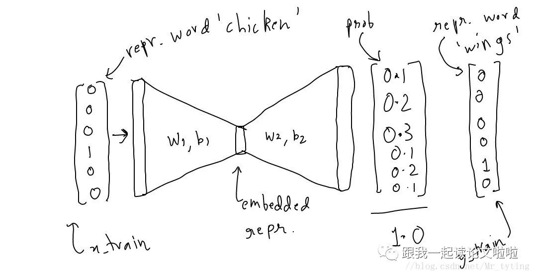
input_one_hot  --->  embedded repr. ---> predicted_neighbour_prob
predicted_prob will be compared against a one hot vector to correct it.

好了，来看看怎么训这个模型

sess = tf.Session()
init = tf.global_variables_initializer()
sess.run(init) #make sure you do this!
# define the loss function:
cross_entropy_loss = tf.reduce_mean(-tf.reduce_sum(y_label * tf.log(prediction), reduction_indices=[1]))
# define the training step:
train_step = tf.train.GradientDescentOptimizer(0.1).minimize(cross_entropy_loss)
n_iters = 10000
# train for n_iter iterations
for _ in range(n_iters):
    sess.run(train_step, feed_dict={x: x_train, y_label: y_train})
    print('loss is : ', sess.run(cross_entropy_loss, feed_dict={x: x_train, y_label: y_train}))

在训的过程中，你可以看到的变化：

loss is :  2.73213
loss is :  2.30519
loss is :  2.11106
loss is :  1.9916
loss is :  1.90923
loss is :  1.84837
loss is :  1.80133
loss is :  1.76381
loss is :  1.73312
loss is :  1.70745
loss is :  1.68556
loss is :  1.66654
loss is :  1.64975
loss is :  1.63472
loss is :  1.62112
loss is :  1.6087
loss is :  1.59725
loss is :  1.58664
loss is :  1.57676
loss is :  1.56751
loss is :  1.55882
loss is :  1.55064
loss is :  1.54291
loss is :  1.53559
loss is :  1.52865
loss is :  1.52206
loss is :  1.51578
loss is :  1.50979
loss is :  1.50408
loss is :  1.49861
.
.
.

最终会收敛，即使其不能达到很高的水平，我们并不这点，我们最终的目的是获取较好的和，也就是。

为什么是？

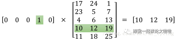
当我们用向量乘以时，获取的是矩阵的某一行，所以扮演的是一个。

在我们这个代码例子中，可以看看在中的。

print(vectors[ word2int['queen'] ])
# say here word2int['queen'] is 2
->
[-0.69424796 -1.67628145  3.07313657 -1.14802659 -1.2207377 ]

给定一个向量，我们可以获取与其最近的向量

def euclidean_dist(vec1, vec2):
    return np.sqrt(np.sum((vec1-vec2)**2))

def find_closest(word_index, vectors):
    min_dist = 10000 # to act like positive infinity
    min_index = -1
    query_vector = vectors[word_index]
    for index, vector in enumerate(vectors):
        if euclidean_dist(vector, query_vector) < min_dist and not np.array_equal(vector, query_vector):
            min_dist = euclidean_dist(vector, query_vector)
            min_index = index
    return min_index

我们来看看，与最近的词：

print(int2word[find_closest(word2int['king'], vectors)])
print(int2word[find_closest(word2int['queen'], vectors)])
print(int2word[find_closest(word2int['royal'], vectors)])
->
queen
king
he

进阶

上面总结的主要是第一篇论文内的内容，虽然只是一个三层的神经网络，但是在海量训练数据的情况下，需要极大的计算资源来支撑整个过程，举例来说，我们设定的时，而时，这时矩阵的维度就达到了！！，这个时候再用来优化训练过程就显得十分缓慢，但是有时候你必须使用大量的数据来训练模型来避免过拟合。论文介绍了几种解决办法。

降采样：采用下采样来降低训练样本数量在里面实现的，并不是所有的的数量，而且先统计了所有的出现频次，然后选取出现频次最高的前的词作为词袋。具体操作请看代码 tensorflow/examples/tutorials/word2vec/word2vec_basic.py^[2]，其余的词用代替。
负采样：采用一种所谓的"负采样"的操作，这种操作每次可以让一个样本只更新权重矩阵中一小部分，减小训练过程中的计算压力。举例来说：一个如：，由上面的分析可知，其为一个向量，并且该向量只是在的位置为 1，其余的位置均为 0，并且该向量的长度为，由此每个样本都缓慢能更新权重矩阵，而"负采样"操作只是随机选择其余的部分，使得其在的位置为 0，那么我们只更新对应位置的权重。例如我们如果选择负采样数量为５，则选取５个其余的，使其对应的为 0，这个时候只是６个神经元，本来我们一次需要更新参数，进行负采样操作以后只需要更新个参数。
Hierarchical Softmax ：是 NLP 中常用方法，详情可以查看Hierarchical Softmax ^[3]。其主要思想是以词频构建 Huffman 树，树的叶子节点为词表中的词，相应的高频词距离根结点更近。当需要计算生成某个词的概率时，不需要对所有词进行概率计算，而是选择在 Huffman 树中从根结点到该词所在结点的路径进行计算，得到生成该词的概率，时间复杂度从 O(N) 降低到 O(logN)（N 个结点，则树的深度 logN）

个人总结

seq2seq 模型，输入处都会乘以，输出处都会乘以，这两个 embedding 矩阵有时会共享，有时则不会。我认为其实就是模型的原型，只不过应用到了不同的复杂场景中，根据场景需要，在内部加了等机制，大致框架依然是。
是当前自然语言处理领域的最基础知识，深刻理解原理非常重要。

完整代码：

import tensorflow as tf
import numpy as np

corpus_raw = 'He is the king . The king is royal . She is the royal  queen '

# convert to lower case
corpus_raw = corpus_raw.lower()

words = []
for word in corpus_raw.split():
    if word != '.': # because we don't want to treat . as a word
        words.append(word)

words = set(words) # so that all duplicate words are removed
word2int = {}
int2word = {}
vocab_size = len(words) # gives the total number of unique words

for i,word in enumerate(words):
    word2int[word] = i
    int2word[i] = word

# raw sentences is a list of sentences.
raw_sentences = corpus_raw.split('.')
sentences = []
for sentence in raw_sentences:
    sentences.append(sentence.split())

WINDOW_SIZE = 2

data = []
for sentence in sentences:
    for word_index, word in enumerate(sentence):
        for nb_word in sentence[max(word_index - WINDOW_SIZE, 0) : min(word_index + WINDOW_SIZE, len(sentence)) + 1] :
            if nb_word != word:
                data.append([word, nb_word])

# function to convert numbers to one hot vectors
def to_one_hot(data_point_index, vocab_size):
    temp = np.zeros(vocab_size)
    temp[data_point_index] = 1
    return temp

x_train = [] # input word
y_train = [] # output word

for data_word in data:
    x_train.append(to_one_hot(word2int[ data_word[0] ], vocab_size))
    y_train.append(to_one_hot(word2int[ data_word[1] ], vocab_size))

# convert them to numpy arrays
x_train = np.asarray(x_train)
y_train = np.asarray(y_train)

# making placeholders for x_train and y_train
x = tf.placeholder(tf.float32, shape=(None, vocab_size))
y_label = tf.placeholder(tf.float32, shape=(None, vocab_size))

EMBEDDING_DIM = 5 # you can choose your own number
W1 = tf.Variable(tf.random_normal([vocab_size, EMBEDDING_DIM]))
b1 = tf.Variable(tf.random_normal([EMBEDDING_DIM])) #bias
hidden_representation = tf.add(tf.matmul(x,W1), b1)

W2 = tf.Variable(tf.random_normal([EMBEDDING_DIM, vocab_size]))
b2 = tf.Variable(tf.random_normal([vocab_size]))
prediction = tf.nn.softmax(tf.add( tf.matmul(hidden_representation, W2), b2))


sess = tf.Session()
init = tf.global_variables_initializer()
sess.run(init) #make sure you do this!

# define the loss function:
cross_entropy_loss = tf.reduce_mean(-tf.reduce_sum(y_label * tf.log(prediction), reduction_indices=[1]))

# define the training step:
train_step = tf.train.GradientDescentOptimizer(0.1).minimize(cross_entropy_loss)

n_iters = 10000
# train for n_iter iterations

for _ in range(n_iters):
    sess.run(train_step, feed_dict={x: x_train, y_label: y_train})
    print('loss is : ', sess.run(cross_entropy_loss, feed_dict={x: x_train, y_label: y_train}))

vectors = sess.run(W1 + b1)

def euclidean_dist(vec1, vec2):
    return np.sqrt(np.sum((vec1-vec2)**2))

def find_closest(word_index, vectors):
    min_dist = 10000 # to act like positive infinity
    min_index = -1
    query_vector = vectors[word_index]
    for index, vector in enumerate(vectors):
        if euclidean_dist(vector, query_vector) < min_dist and not np.array_equal(vector, query_vector):
            min_dist = euclidean_dist(vector, query_vector)
            min_index = index
    return min_index


from sklearn.manifold import TSNE

model = TSNE(n_components=2, random_state=0)
np.set_printoptions(suppress=True)
vectors = model.fit_transform(vectors)

from sklearn import preprocessing

normalizer = preprocessing.Normalizer()
vectors =  normalizer.fit_transform(vectors, 'l2')

print(vectors)

import matplotlib.pyplot as plt


fig, ax = plt.subplots()
print(words)
for word in words:
    print(word, vectors[word2int[word]][1])
    ax.annotate(word, (vectors[word2int[word]][0],vectors[word2int[word]][1] ))
plt.show()

参考资料

[1]

Word2Vec Tutorial - The Skip-Gram Model: http://mccormickml.com/2016/04/19/word2vec-tutorial-the-skip-gram-model/

[2]

tensorflow/examples/tutorials/word2vec/word2vec_basic.py: https://www.github.com/tensorflow/tensorflow/blob/r1.7/tensorflow/examples/tutorials/word2vec/word2vec_basic.py

[3]

Hierarchical Softmax : https://blog.csdn.net/itplus/article/details/37969979

本文转载自公众号：跟我一起读论文啦啦，作者：村头陶员外

推荐阅读

BERT论文总结

BERT系列文章汇总导读

BERT 瘦身之路：Distillation，Quantization，Pruning

BERT论文笔记

BERT 的演进和应用

关于AINLP

AINLP 是一个有趣有AI的自然语言处理社区，专注于 AI、NLP、机器学习、深度学习、推荐算法等相关技术的分享，主题包括文本摘要、智能问答、聊天机器人、机器翻译、自动生成、知识图谱、预训练模型、推荐系统、计算广告、招聘信息、求职经验分享等，欢迎关注！加技术交流群请添加AINLP君微信(id：AINLP2)，备注工作/研究方向+加群目的。

登录查看更多

相关内容

词向量表示

关注 37

分散式表示即将语言表示为稠密、低维、连续的向量。研究者最早发现学习得到词嵌入之间存在类比关系。比如apple−apples ≈ car−cars， man−woman ≈ king – queen 等。这些方法都可以直接在大规模无标注语料上进行训练。词嵌入的质量也非常依赖于上下文窗口大小的选择。通常大的上下文窗口学到的词嵌入更反映主题信息，而小的上下文窗口学到的词嵌入更反映词的功能和上下文语义信息。

最新《图神经网络知识图谱补全》综述论文

专知会员服务

157+阅读 · 2020年7月29日

KG-BERT：基于BERT的知识图谱补全，KG-BERT: BERT for Knowledge Graph Completion

专知会员服务

195+阅读 · 2020年5月31日

超越三元组:基于超关系知识图谱嵌入的链接预测，Beyond Triplets: Hyper-Relational Knowledge Graph Embedding for Link Prediction

专知会员服务

78+阅读 · 2020年5月11日