实战 | 手把手教你用PyTorch实现图像描述（附完整代码）

2018 年 5 月 9 日 人工智能头条 爱技术

作者 | 李理

环信人工智能研发中心 VP，十多年自然语言处理和人工智能研发经验。主持研发过多款智能硬件的问答和对话系统，负责环信中文语义分析开放平台和环信智能机器人的设计与研发。

想要详细了解该系列文章，营长建议你先阅读上篇：一文详解循环神经网络的基本概念（代码版）

Tensor

和TensorFlow 类似，PyTorch 的核心对象也是Tensor。下面是创建Tensor 的代码：

x = torch.Tensor(5, 3)
print(x)

对应的下标是5，那么在这个下标的值为1，而其余的值为0，因此一个词只有一个位置不为0，所以叫作one-hot 的表示方法。这种表示方法的缺点是它是一种“稀疏”的表示方法，两个词，不论语义是相似还是不同，都无法通过这个向量表示出来。比如我们计算两个向量的内积，相同的词内积为1（表示相似度很高）；而不同的词为0（表示完全不同）。但实际我们希望“猫”和“狗”的相似度要高于“猫”和“石头”，使用one-hot 就无法表示出来。

Word Embedding 的思想是把高维的稀疏向量映射到一个低维的稠密向量，要求是两个相似的词会映射到低维空间里距离比较近的两个点；而不相似的距离较远。我们可以这样来“理解”这个低维的向量——假设语义可以用n 个基本的“正交”的“原子”语义表示的话，那么向量的不同的维代表这个词在这个原子语义上的“多少”。

当然这只是一种假设，但实际这个语义空间是否存在，或者即使存在也可能和人类理解的不同，但是只要能达到前面的要求——相似的词的距离近而不相似的远，也就可以了。

举例来说，假设向量的第一维表示动物，那么猫和狗应该在这个维度上有较大的值，而石头应该较小。

Embedding 一般有两种方式得到，一种是通过与任务无直接关系的无监督任务中学习，比如早期的RNN 语言模型，它的一个副产品就是Word Embedding，包括后来的专门Embedding 方法如Word to Vector 或者GloVe 等，本书后面的章节会详细介绍。另外一种方式就是在当前任务中让它自己学习出最合适的Word Embedding来。前一种方法的好处是可以利用海量的无监督数据，但是由于领域有差别以及它不是针对具体任务的最优化表示，它的效果可能不会很好；而后一种方法它针对当前任务学习出最优的表示（和模型的参数配合），但是它需要海量的训练数据，这对很多任务来说是无法满足的条件。在实践中，如果领域的数据非常少，我们可能直接用在其它任务中Pretraining 的Embedding 并且fix 住它；而如果领域数据较多的时候我们会用Pretraining 的Embedding 作为初始值，然后用领域数据驱动它进行微调。

PyTorch 基础知识

▌Tensor

和TensorFlow 类似，PyTorch 的核心对象也是Tensor。下面是创建Tensor 的代码：

x = torch.Tensor(5, 3)
print(x)

输出：

0.2455 0.1516 0.5319
0.9866 0.9918 0.0626
0.0172 0.6471 0.1756
0.8964 0.7312 0.9922
0.6264 0.0190 0.0041
[torch.FloatTensor of size 5x3]

我们可以得到Tensor 的大小：

print(x.size())
输出：
torch.Size([5, 3])

▌Operation

和TensorFlow 一样，有了Tensor 之后就可以用Operation 进行计算了。但是和TensorFlow 不同，TensorFlow 只是定义计算图但不会立即“执行”，而Pytorch 的Operation 是马上“执行”的。所以PyTorch 使用起来更加简单，当然PyTorch 也有计算图的执行引擎，但是它不对用户可见，它是“动态”编译的。

首先是加分操作：

y = torch.rand(5, 3)
print(x + y)

上面的加法会产生一个新的Tensor，但是我们可以提前申请一个Tensor 来存储Operation 的结果：

result = torch.Tensor(5, 3)
torch.add(x, y, out=result)
print(result)

也可以in-place 的修改：

# adds x to y
y.add_(x)
print(y)

一般来说，如果一个方法已_ 结尾，那么这个方法一般来说就是in-place 的函数。

PyTorch 支持numpy 的索引操作，比如取第一列：

print(x[:, 1])

我们也可以用view 来修改Tensor 的shape，注意view 要求新的Tensor 的元素个数和原来是一样的。

x = torch.randn(4, 4)
y = x.view(16)
z = x.view(-1, 8) # the size -1 is inferred from other dimensions
print(x.size(), y.size(), z.size())
输出：torch.Size([4, 4]) torch.Size([16]) torch.Size([2, 8])

▌numpy ndarray 的转换

我们可以很方便的把Tensor 转换成numpy 的ndarray 或者转换回来，注意它们是共享内存的，修改Tensor 会影响numpy 的ndarray，反之亦然。

Tensor 转numpy

a = torch.ones(5)
b = a.numpy()
a.add_(1) # 修改a会影响b

numpy 转Tensor

import numpy as np
a = np.ones(5)
b = torch.from_numpy(a)
np.add(a, 1, out=a) # 修改a会影响b

▌CUDA Tensor

Tensor 可以移到GPU 上用GPU 来加速计算：

# let us run this cell only if CUDA is available
if torch.cuda.is_available():
x = x.cuda()
y = y.cuda()
x + y 在GPU上计算

图5.18: PyTorch 的变量

▌Autograd

autograd 是PyTorch 核心的包，用于实现前面我们提到的自动梯度算法。首先我们介绍其中的变量。

▌Variable

autograd.Variable 是Tensor 的封装，我们定义（也就计算）好了最终的变量(一般是Loss) 后，我们可以调用它的backward() 方法，PyTorch 就会自动的计算好梯度。如图5.18所示，PyTorch 的变量值会存储到data 里，而梯度值会存放到grad 里，此外还有一个grad_fn，它是用来计算梯度的函数。除了用户创建的Tensor 之外，通过Operatioon 创建的变量会记住它依赖的变量，从而形成一个有向无环图。计算这个变量的梯度的时候会自动计算它依赖的变量的梯度。

我们可以这样定义变量，参数requires_grad 说明这个变量是否参与计算梯度：

x = Variable(torch.ones(2, 2), requires_grad=True)

▌Gradient

我们可以用backward() 来计算梯度，它等价于variable.backward(torch.Tensor([1.0]))，梯度会往后往前传递，最后的变量一般传递的就是1，然后往前计算梯度的时候会把之前的值累积起来，PyTorch 会自动处理这些东西，我们不需要考虑。

x = Variable(torch.ones(2, 2), requires_grad=True)
y=x+2
z = y * y * 3
out = z.mean()
out.backward() # 计算所有的dout/dz,dout/dy,dout/dx
print(x.grad) # x.grad就是dout/dx
输出为：
4.5000 4.5000
4.5000 4.5000
[torch.FloatTensor of size 2x2]

我们手动来验证一下：

注意每次调用backward() 都会计算梯度然后累加到原来的值之上，所以如果每次计算梯度之前要调用变量的zero_grad() 函数。

▌变量的requires_grad 和volatile

每个变量有两个flag：requires_grad 和volatile，它们可以细粒度的控制一个计算图的某个子图不需要计算梯度，从而可以提高计算速度。一个Operation 如果所有的输入都不需要计算梯度(requires_grad==False)，那么这个Operation 的requires_grad就是False，而只要有一个输入，那么这个Operation 就需要计算梯度。比如下面的代码片段：

>>> x = Variable(torch.randn(5, 5))
>>> y = Variable(torch.randn(5, 5))
>>> z = Variable(torch.randn(5, 5), requires_grad=True)
>>> a = x + y
>>> a.requires_grad
False
>>> b = a + z
>>> b.requires_grad
True

如果你想固定住模型的某些参数，或者你知道某些参数的梯度不会被用到，那么就可以把它们的requires_grad 设置成False。比如我们想细调(fine-tuing) 预先训练好的一个CNN，我们会固定所有最后全连接层之前的卷积池化层参数，我们可以这样：

model = torchvision.models.resnet18(pretrained=True)
for param in model.parameters():
   param.requires_grad = False
   
# 把最后一个全连接层替换成新构造的全连接层
# 默认的情况下，新构造的模块的requires_grad=True
model.fc = nn.Linear(512, 100)

# 优化器只调整新构造的全连接层的参数。
optimizer = optim.SGD(model.fc.parameters(), lr=1e-2, momentum=0.9)

volatile 在0.4.0 之后的版本以及deprecated 了，不过我们后面的代码会用到它之前的版本，因此还是需要了解一下。它适用于预测的场景，在这里完全不需要调用backward() 函数。它比requires_grad 更加高效，而且如果volatile 是True，那么它会强制requires_grad 也是True。它和requires_grad 的区别在于：如果一个Operation的所有输入的requires_grad 都是False 的时候，这个Operation 的requires_grad 才是False，这时这个Operation 就不参与梯度的计算；而如果一个Operation 的一个输入是volatile 是True，那么这个Operation 的volatile 就是True 了，那么这个Operation 就不参与梯度的计算了。因此它很适合的预测场景时：不修改模型的任何定义，只是把输入变量（的一个）设置成volatile，那么计算forward 的时候就不会保留任何用于backward 的中间结果，这样就会极大的提高预测的速度。下面是示例代码：

>>> regular_input = Variable(torch.randn(1, 3, 227, 227))
>>> volatile_input = Variable(torch.randn(1, 3, 227, 227), volatile=True)
>>> model = torchvision.models.resnet18(pretrained=True)
>>> model(regular_input).requires_grad
True
>>> model(volatile_input).requires_grad
False
>>> model(volatile_input).volatile
True
>>> model(volatile_input).grad_fn is None
True

图5.19: 卷积网络

▌神经网络

有了前面的变量和梯度计算，理论上我们就可以自己实现各种深度学习算法，但用户会有很多重复的代码，因此PyTorch 提供了神经网络模块torch.nn。在实际的PyTorch 开发中，我们通过继承nn.Module 来定义一个网络，我们一般值需要实现forward() 函数，而PyTorch 自动帮我们计算backward 的梯度，此外它还提供了常见的Optimizer 和Loss，减少我们的重复劳动。我们下面会实现如图5.19的卷积网络，因为之前已经详细的介绍了理论的部分，我们这里只是简单的介绍怎么用PyTorch 来实现。

完整代码：

https://github.com/fancyerii/deep_learning_theory_and_practice/

blob/master/codes/ch05/PyTorch%20CNN.ipynb

对于PyTorch 的开发来说，一般是如下流程：

定义网络可训练的参数
变量训练数据
forward 计算loss
backward 计算梯度
更新参数，比如weight = weight - learning_rate * gradient

下面我们按照前面的流程来实现这个卷积网络。

定义网络

import torch
from torch.autograd import Variable
import torch.nn as nn
import torch.nn.functional as F

class Net(nn.Module): # 必须集成nn.Module
    def __init__(self):
       super(Net, self).__init__() # 必须调用父类的构造函数，传入类名和self
       # 输入是1个通道(灰度图)，卷积feature
           map的个数是6，大小是5x5，无padding，stride是1。
       self.conv1 = nn.Conv2d(1, 6, 5)
       # 第二个卷积层feature map个数是16，大小还是5*5，无padding，stride是1。
self.conv2 = nn.Conv2d(6, 16, 5)
       # 仿射层y = Wx + b，ReLu层没有参数，因此不在这里定义
self.fc1 = nn.Linear(16 * 5 * 5, 120)
self.fc2 = nn.Linear(120, 84)
self.fc3 = nn.Linear(84, 10)

def forward(self, x):
    # 卷积然后Relu然后2x2的max pooling
    x = F.max_pool2d(F.relu(self.conv1(x)), (2, 2))
    # 再一层卷积relu和max pooling
    x = F.max_pool2d(F.relu(self.conv2(x)), 2)
    # 把batch x channel x width x height 展开成batch x all_nodes
    x = x.view(-1, self.num_flat_features(x))
    x = F.relu(self.fc1(x))
    x = F.relu(self.fc2(x))
    x = self.fc3(x)
    return x

def num_flat_features(self, x):
    size = x.size()[1:] # 除了batchSize之外的其它维度
    num_features = 1
    for s in size:
        num_features *= s
     return num_features

net = Net()

print(net)

输出为：

Net(
  (conv1): Conv2d (1, 6, kernel_size=(5, 5), stride=(1, 1))
  (conv2): Conv2d (6, 16, kernel_size=(5, 5), stride=(1, 1))
  (fc1): Linear(in_features=400, out_features=120)
  (fc2): Linear(in_features=120, out_features=84)
  (fc3): Linear(in_features=84, out_features=10)
)

我们值需要实现forward() 函数，PyTorch 会自动帮我们实现backward() 和梯度计算。我们可以列举net 的所有可以训练的参数，前面我们在Net 里定义的所有变量都会保存在net 的parameters 里。

params = list(net.parameters())
print(len(params))
print(params[0].size()) # conv1's .weight
10
torch.Size([6, 3, 5, 5])

代码要求forward 的输入是一个变量(不需要梯度)，它的大小是batch x 1 x 32 x 32。

input = Variable(torch.randn(1, 1, 32, 32))
out = net(input)
print(out)

注意，我们直接调用net(input)，不需要显式调用forward() 方法。我们可以调用backward() 来计算梯度，调用前记得调用zero_grad。

net.zero_grad()
out.backward(torch.randn(1, 10))

nn.Conv2d() 只支持batch 的输入，如果只有一个数据，也要转成batchSize 为1 的输入。如果输入是channel x width x height，我们可以使用input.unsqueeze(0) 把它变成1 x channel x width x height 的。

损失函数

接下来我们会定义损失函数，PyTorch 为我们提供了很多常见的损失函数，比如

MSELoss：

output = net(input)
target = Variable(torch.arange(1, 11)) # 只是示例
criterion = nn.MSELoss()
loss = criterion(output, target)
print(loss)

如果我们沿着loss 从后往前用grad_fn 函数查看，可以得到如下：

input -> conv2d -> relu -> maxpool2d -> conv2d -> relu -> maxpool2d
-> view -> linear -> relu -> linear -> relu -> linear
-> MSELoss
-> loss

我们可以用next_function 来查看之前的grad_fn。

print(loss.grad_fn) # MSELoss
print(loss.grad_fn.next_functions[0][0]) # Linear
print(loss.grad_fn.next_functions[0][0].next_functions[0][0]) # ReLU

梯度计算

有了Loss 之后我们就可以计算梯度：

net.zero_grad() # 记得清零。
print('conv1.bias.grad before backward')
print(net.conv1.bias.grad)
loss.backward()
print('conv1.bias.grad after backward')
print(net.conv1.bias.grad)

更新参数

我们可以自己更新参数：weight = weight - learning_rate * gradient。比如代码：

learning_rate = 0.01
for f in net.parameters():
f.data.sub_(f.grad.data * learning_rate)

但是除了标准的SGD 算法，我们前面还介绍了很多算法比如Adam 等，没有必要让大家自己实现，所以PyTorch 提供了常见的算法，包括SGD：

import torch.optim as optim
# 创建optimizer
optimizer = optim.SGD(net.parameters(), lr=0.01)
# 训练循环
optimizer.zero_grad() # 清零
output = net(input)
loss = criterion(output, target)
loss.backward()
optimizer.step() # 更新参数

数据集和transforms

对于常见的MNIST 和CIFAR-10 数据集，PyTorch 自动提供了下载和读取的代码：

transform = transforms.Compose(
[transforms.ToTensor(),
transforms.Normalize((0.5, 0.5, 0.5), (0.5, 0.5, 0.5))])

trainset = torchvision.datasets.CIFAR10(root='./data', train=True,
download=True, transform=transform)
trainloader = torch.utils.data.DataLoader(trainset, batch_size=4,
shuffle=True, num_workers=2)

testset = torchvision.datasets.CIFAR10(root='./data', train=False,
download=True, transform=transform)
testloader = torch.utils.data.DataLoader(testset, batch_size=4,
shuffle=False, num_workers=2)

这里有个transform，datasets.CIFAR10 返回的是PIL 的[0,1] 的RGB 值，我们首先转成Tensor，然后在把它转换成[-1,1] 区间的值。transforms.Normalize(0.5,0.5) 会用如下公式进行归一化：

input[channel] = (input[channel] − mean[channel])/std[channel]

对于上面的取值input=(input-0.5)*2，也就是把范围从[0,1] 变成[-1,1]。关于Dataset和DataLoader 更多细节，请参考完整代码。

完整代码在ch05/PyTorch CNN.ipynb。我们这里的目的只是介绍PyTorch 的基本概念，因此使用了最简单的CNN。

PyTorch 循环网络示例

接下来我们通过几个示例介绍怎么在 PyTorch 里使用卷积网络。

▌姓名分类

这个示例会构建一个分类器，输入是一个姓名，输出是这个姓名的人可能来自哪个国家。我们下面会训练一个字符级别的RNN 模型来预测一个姓名是哪个国家人的姓名。我们的数据集收集了18 个国家的近千个人名(英文名，注意中国人也是英文名，否则就是语言识别问题了），我们最终的模型就可以预测这个姓名是哪个国家的人。

完整代码在

https://github.com/fancyerii/deep_learning_theory_and_practice/blob/

master/codes/ch05/Char%20RNN%20Classifier.ipynb

数据准备

在data/names 目录下有18 个文本文件，命名规范为[语言].txt。每个文件的每一行都是一个人名。此外，我们实现了一个unicode_to_ascii 把诸如à 之类转换成a。最终我们得到一个字典category_lines，language: [names ...]。key 是语言名，value 是名字的列表。all_letters 里保存所有的字符。

import glob

all_filenames = glob.glob('../data/names/*.txt')
print(all_filenames)

import unicodedata
import string

all_letters = string.ascii_letters + " .,;'"
n_letters = len(all_letters)

# http://stackoverflow.com/a/518232/2809427
def unicode_to_ascii(s):
   return ''.join(
       c for c in unicodedata.normalize('NFD', s)
       if unicodedata.category(c) != 'Mn'
       and c in all_letters
)

print(unicode_to_ascii('Ślusàrski'))

category_lines = {}
all_categories = []

def readLines(filename):
   lines = open(filename).read().strip().split('\n')
   return [unicode_to_ascii(line) for line in lines]

for filename in all_filenames:
   category = filename.split('/')[-1].split('.')[0]
   all_categories.append(category)
   lines = readLines(filename)
   category_lines[category] = lines
   
n_categories = len(all_categories)
print('n_categories =', n_categories)

把姓名(String) 变成Tensor

现在我们已经把数据处理好了，接下来需要把姓名从字符串变成Tensor，因为机器学习只能处理数字。为了表示一个字母，我们使用“one-hot” 的表示方法。这是一个长度为<1 x n_letters> 的向量，对应字符的下标为1，其余为0。对于一个姓名，我们用大小为<line_length x 1 x n_letters> 的Tensor 来表示。第二维表示batch 大小，因为PyTorch 的RNN 要求输入是< time x batch x input_features>。

import torch

# 把一个字母变成<1 x n_letters> Tensor
def letter_to_tensor(letter):
    tensor = torch.zeros(1, n_letters)
    letter_index = all_letters.find(letter)
    tensor[0][letter_index] = 1
    return tensor

# 把一行(名字)转换成<line_length x 1 x n_letters>的Tensor
def line_to_tensor(line):
    tensor = torch.zeros(len(line), 1, n_letters)
    for li, letter in enumerate(line):
        letter_index = all_letters.find(letter)
        tensor[li][0][letter_index] = 1
return tensor

创建网络

如果想“手动”创建网络，那么在PyTorch 里创建RNN 和全连接网络的代码并没有太大差别。因为PyTorch 的计算图是动态实时编译的，不同time-step 的for 循环不需要“内嵌”在RNN 里。因此每个训练数据即使长度不同也没有关系，因为每次都是根据当前的数据长度“实时”编译出来的计算图。网络结构如下图所示：

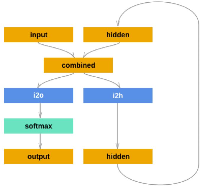
图5.20: RNN 分类器网络结构

这个网络结构和vanilla RNN 的区别在于我们使用了两个全连接层，一个用于计算新的hidden；另一个用于计算当前的输出。而在vanilla RNN 中只有一个全连接层计算hidden，同时用这个hidden 计算输出。定义网络的代码如下：

import torch.nn as nn
from torch.autograd import Variable

class RNN(nn.Module):
    def __init__(self, input_size, hidden_size, output_size):
        super(RNN, self).__init__()

self.input_size = input_size
self.hidden_size = hidden_size
self.output_size = output_size

self.i2h = nn.Linear(input_size + hidden_size, hidden_size)
self.i2o = nn.Linear(input_size + hidden_size, output_size)
self.softmax = nn.LogSoftmax(dim=1)

def forward(self, input, hidden):
   combined = torch.cat((input, hidden), 1)
   hidden = self.i2h(combined)
   output = self.i2o(combined)
   output = self.softmax(output)
   return output, hidden
def init_hidden(self):
   return Variable(torch.zeros(1, self.hidden_size))

和之前的全连接网络一样，首先我们的类需要基础nn.Module 并且实现

__init__、forward 和init_hidden 这3 个方法。在__init__ 方法里，我们定

义网络中的变量，以及两个全连接层。forward 函数根据当前的输入input 和上一个时刻的hidden 计算新的输出和hidden。init_hidden 创建一个初始为0 的隐状态。

测试网络

定义好了网络之后我们可以测试一下：

n_hidden = 128
rnn = RNN(n_letters, n_hidden, n_categories)

input = Variable(line_to_tensor('Albert'))
hidden = Variable(torch.zeros(1, n_hidden))

# 实际是遍历所有input
output, next_hidden = rnn(input[0], hidden)
print(output)
hidden=net_hidden

准备训练

测试没什么问题之后就可以开始训练了。训练之前，我们需要一些工具函数。第一个就是根据网络的输出把它变成分类，我们这里使用Tensor.topk 来选取概率最大的那个下标，然后得到分类名称。

def category_from_output(output):
   top_n, top_i = output.data.topk(1) # Tensor out of Variable with .data
   category_i = top_i[0][0]
   return all_categories[category_i], category_i
   
print(category_from_output(output))

我们也需要一个函数来随机挑选一个训练数据：

import random

def random_training_pair():
   category = random.choice(all_categories)
   line = random.choice(category_lines[category])
   category_tensor =
       Variable(torch.LongTensor([all_categories.index(category)]))
   line_tensor = Variable(line_to_tensor(line))
   return category, line, category_tensor, line_tensor

for i in range(10):
   category, line, category_tensor, line_tensor = random_training_pair()
   print('category =', category, '/ line =', line)

训练

现在我们可以训练网络了，因为RNN 的输出已经取过log 了，所以计算交叉熵只需要选择正确的分类对于的值就可以了，PyTorch 提供了nn.NLLLoss() 函数来实现这个目的，它基本就是实现了loss(x, class) = -x[class]。

criterion = nn.NLLLoss()

我们可以用optimizer 而不是自己手动来更新参数，这里我们使用最原始的SGD 算法。

learning_rate = 0.005
optimizer = torch.optim.SGD(rnn.parameters(), lr=learning_rate)

训练的每个循环如下：创建输入和输出Tensor 创建初始化为零的隐状态Tensor for each letter in 输入Tensor: output, hidden=rnn(input,hidden) 计算loss backward 计算梯度optimizer.step

def train(category_tensor, line_tensor):
   rnn.zero_grad()
   hidden = rnn.init_hidden()

for i in range(line_tensor.size()[0]):
   output, hidden = rnn(line_tensor[i], hidden)

loss = criterion(output, category_tensor)
loss.backward()

optimizer.step()
return output, loss.data[0]

接下来我们就要用训练数据来训练了。因为上面的函数同时返回输出和损失，我们可以保存下来用于绘图。

import time
import math

n_epochs = 100000
print_every = 5000
plot_every = 1000

current_loss = 0
all_losses = []

def time_since(since):
   now = time.time()
   s = now - since
   m = math.floor(s / 60)
   s -= m * 60
   return '%dm %ds' % (m, s)

start = time.time()

for epoch in range(1, n_epochs + 1):
   # 随机选择一个样本
   category, line, category_tensor, line_tensor = random_training_pair()
   output, loss = train(category_tensor, line_tensor)
   current_loss += loss
   
   if epoch % print_every == 0:
     guess, guess_i = category_from_output(output)
     correct = '􀀀' if guess == category else '􀀀 (%s)' % category
     print('%d %d%% (%s) %.4f %s / %s %s' % (epoch, epoch / n_epochs * 100,
         time_since(start), loss, line, guess, correct))

if epoch % plot_every == 0:
  all_losses.append(current_loss / plot_every)
current_loss = 0

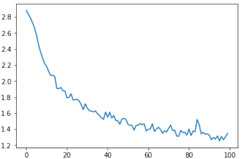
图5.21: 训练的损失

绘图

把所有的损失都绘制出来可以显示学习的过程。

import matplotlib.pyplot as plt
import matplotlib.ticker as ticker
%matplotlib inline


plt.figure()
plt.plot(all_losses)

评估效果

为了查看模型的效果，我们需要创建一个混淆矩阵，每一行代表样本实际的类别，而每一列表示模型预测的类别。为了计算混淆矩阵，我们需要使用evaluate 方法来预测，它和train() 基本一样，只是少了反向计算梯度的过程。

# 混淆矩阵
confusion = torch.zeros(n_categories, n_categories)
n_confusion = 10000

def evaluate(line_tensor):
  hidden = rnn.init_hidden()

  for i in range(line_tensor.size()[0]):
     output, hidden = rnn(line_tensor[i], hidden)

     return output
     
# 最好是有一个测试数据集，我们这里随机从训练数据里采样
for i in range(n_confusion):
   category, line, category_tensor, line_tensor = random_training_pair()
   output = evaluate(line_tensor)
   guess, guess_i = category_from_output(output)
   category_i = all_categories.index(category)
   confusion[category_i][guess_i] += 1

# 归一化
for i in range(n_categories):
   confusion[i] = confusion[i] / confusion[i].sum()
   
fig = plt.figure()
ax = fig.add_subplot(111)
cax = ax.matshow(confusion.numpy())
fig.colorbar(cax)

# 设置x轴的文字往上走
ax.set_xticklabels([''] + all_categories, rotation=90)
ax.set_yticklabels([''] + all_categories)
ax.xaxis.set_major_locator(ticker.MultipleLocator(1))
ax.yaxis.set_major_locator(ticker.MultipleLocator(1))

plt.show()

最终的混淆矩阵如图5.22所示。

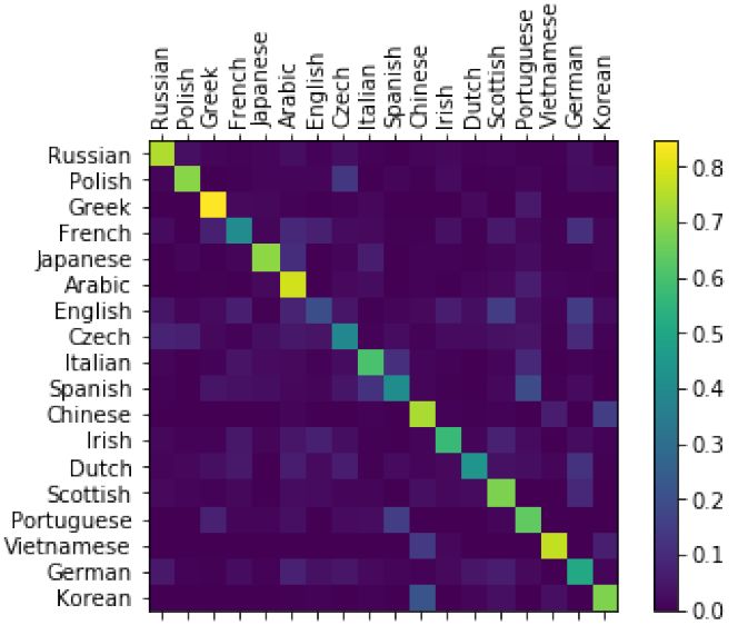
图5.22: 混淆矩阵

测试

我们首先实现predict 函数，它会预测输入名字概率最大的3 个国家。然后手动输入几个训练数据里不存在的人名进行测试。

def predict(input_line, n_predictions=3):
   print('\n> %s' % input_line)
   output = evaluate(Variable(line_to_tensor(input_line)))

   topv, topi = output.data.topk(n_predictions, 1, True)
   predictions = []
   
for i in range(n_predictions):
   value = topv[0][i]
   category_index = topi[0][i]
   print('(%.2f) %s' % (value, all_categories[category_index]))
   predictions.append([value, all_categories[category_index]])

predict('Dovesky')
predict('Jackson')
predict('Satoshi')

▌RNN 生成莎士比亚风格句子

这个例子会用莎士比亚的著作来训练一个char-level RNN 语言模型，同时使用它来生成莎士比亚风格的句子。

完整代码:

https://github.com/fancyerii/deep_learning_theory_and_practice/

blob/master/codes/ch05/Char%20RNN%20%E7%94%9F%E6%88%90%E5%99%A8.ipynb

准备数据

输入文件是纯文本文件，我们会使用unidecode 来把unicode 转成ASCII 文本。

import unidecode
import string
import random
import re

all_characters = string.printable
n_characters = len(all_characters)

file = unidecode.unidecode(open('../data/shakespeare.txt').read())
file_len = len(file)
print('file_len =', file_len)

这个文件太大了，我们随机的进行截断来得到一个训练数据。

chunk_len = 200

def random_chunk():
start_index = random.randint(0, file_len - chunk_len)
end_index = start_index + chunk_len + 1
return file[start_index:end_index]

print(random_chunk())

PyTorch 的RNN 简介

之前的Char RNN 分类器，我们是“手动”实现的最朴素的RNN。我们就像实现一个普通的前馈神经网络一样实现RNN，因为我们在for 循环里复用同一个全连接层，因此PyTorch 会自动帮我们展开从而实现BPTT。现在下面的例子里将使用PyTorch提供的GRU 模块，这比我们自己“手动”实现的版本效率更高，也更容易复用。我们下面会简单的介绍PyTorch 中的RNN 相关模块。

1. torch.nn.RNN

这个类用于实现前面介绍的vanilla 的RNN，其具体计算公式为：ht = tanh(wihxt +bih + whhht−1 + bhh)，其中ht 是t 时刻的隐状态，xt 是t 时刻的输入。如果我们想使用其它的激活函数比如ReLu 可以在构造函数里传入nonlinearity=’relu’。构造函数的参数为：

input_size 输入xt 的大小
hidden_size 隐单元的个数
num_layers RNN 的层数，默认1
nonlinearity 激活函数，可以是’tanh’ 或者’relu’，默认是’tanh’
bias 是否有bias
batch_first 如果为True，那么输入要求是(batch, seq, feature)，否则是(seq,batch, feature)，默认是False
dropout dropout 概率。默认0，没有dropout
bidirectional 是否双向RNN。默认False

它的输入是input 和h0 格式如下：

input shape 是(seq_len, batch, input_size)，如果构造参数batch_first 是True，则要求输入是(batch, seq_len, input_size)。
h0 shape 是(num_layers * num_directions, batch, hidden_size)

它的输出是output, hn 格式如下：

output 是最后一层的输出，shape 是(seq_len, batch, hidden_size * num_directions)
hn 的shape 是(num_layers * num_directions, batch, hidden_size)

它包含的变量为：

weight_ih_l[k] 第k 层输入到隐单元的可训练的weight。如果k 是0(第一层)，那么它的shape 是(hidden_size * input_size)，否则是(hidden_size * hidden_size)
weight_hh_l[k] 第k 层(上一个时刻的) 隐单元到隐单元的weight。shape 是(hidden_size * hidden_size)
bias_ih_l[k] 第k 层输入到隐单元的bias。shape 是(hidden_size)
bias_hh_l[k] 第k 层隐单元到隐单元的bias。shape 也是(hidden_size)

代码示例：

>>> rnn = nn.RNN(10, 20, 2)
>>> input = torch.randn(5, 3, 10)
>>> h0 = torch.randn(2, 3, 20)
>>> output, hn = rnn(input, h0)

在上面的例子里，我们定义了一个2 层的(单向)RNN，输入大小是10，隐单元个数是20。输入是(5,3,10)，表示batch 是3；序列长度是5；输入大小是10（这是和前面RNN 的定义匹配的）。h0 是(2,3,20)，第一维是2，表示2 层；第二维是3，表示batch；第三维是20，表示20 个隐单元。

2. torch.nn.LSTM PyTorch 实现的LSTM 计算过程如下：

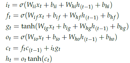
其中，ht 是t 时刻的隐状态，ct 是t 时刻的cell 状态，xt 是t 时刻的输入。it, ft, gt, ot分别是t 时刻的输入门，遗忘门，cell gate 和输出门。构造函数参数如下：

input_size 输入x 的特征维数
hidden_size 隐单元个数
num_layers LSTM 的层数，默认1
bias 是否有bias
batch_first 如果为True，那么输入要求是(batch, seq, feature)，否则是(seq,batch, feature)，默认是False
dropout dropout 概率。默认0，没有dropout
bidirectional 是否双向RNN。默认False

输入input, (h_0, c_0) 格式如下：

input shape 是(seq_len, batch, input_size)，如果构造参数batch_first 是True，则要求输入是(batch, seq_len, input_size)。
h_0 (num_layers * num_directions, batch, hidden_size)
c_0 (num_layers * num_directions, batch, hidden_size)

输出output, (hn, cn) 格式如下：

output 是最后一层LSTM 的输出，shape (seq_len, batch, hidden_size * num_directions)
h_n 隐状态，shape 是(num_layers * num_directions, batch, hidden_size)
c_n cell 状态，shape 是(num_layers * num_directions, batch, hidden_size)

它包含的变量为：

weight_ih_l[k] 第k 层输入到隐单元的可训练的weight。
shape 是(4*hidden_size* input_size)
weight_hh_l[k] 第k 层(上一个时刻的) 隐单元到隐单元的weight。
shape 是(4*hidden_size * hidden_size)
bias_ih_l[k] 第k 层输入到隐单元的bias。
shape 是(4*hidden_size)
bias_hh_l[k] 第k 层隐单元到隐单元的bias。
shape 也是(4*hidden_size)

示例：

>>> rnn = nn.LSTM(10, 20, 2)
>>> input = torch.randn(5, 3, 10)
>>> h0 = torch.randn(2, 3, 20)
>>> c0 = torch.randn(2, 3, 20)
>>> output, hn = rnn(input, (h0, c0))

和前面的RNN 例子类似，只是多了一个h0。

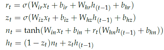
3. torch.nn.GRU GRU 的计算过程如下：

构造函数参数如下：

input_size 输入x 的特征维数
hidden_size 隐单元个数
num_layers LSTM 的层数，默认1
bias 是否有bias
batch_first 如果为True，那么输入要求是(batch, seq, feature)，否则是(seq,batch, feature)，默认是False
dropout dropout 概率。默认0，没有dropout
bidirectional 是否双向RNN。默认False

它的输入是input 和h0 格式如下：

input shape 是(seq_len, batch, input_size)，如果构造参数batch_first 是True，则要求输入是(batch, seq_len, input_size)。
h0 shape 是(num_layers * num_directions, batch, hidden_size)

关于PyTorch 的输出，比如h0 的shape 是(num_layers * num_directions, batch,hidden_size)，虽然文档没有明确说明，但是我们一般可以”猜测“输出的第一维(num_layers * num_directions) 是先num_layers 后num_directions 的。举例来说，如果RNN 是2 层的并且是双向的，那么输出h0 的顺序是这样的：(layer1-正向的隐状态,layer1-逆向的隐状态,layer2-正向的隐状态,layer2-逆向的隐状态)。

它的输出是output, hn 格式如下：

output 是最后一层的输出。
shape 是(seq_len, batch, hidden_size * num_directions)
hn 的shape 是(num_layers * num_directions, batch, hidden_size)

它包含的变量为：

weight_ih_l[k] 第k 层输入到隐单元的可训练的weight。
shape 是(3*hidden_size* input_size)
weight_hh_l[k] 第k 层(上一个时刻的) 隐单元到隐单元的weight。
shape 是(3*hidden_size * hidden_size)
bias_ih_l[k] 第k 层输入到隐单元的bias。
shape 是(3*hidden_size)
bias_hh_l[k] 第k 层隐单元到隐单元的bias。
shape 也是(3*hidden_size)

示例：

>>> rnn = nn.GRU(10, 20, 2)
>>> input = torch.randn(5, 3, 10)
>>> h0 = torch.randn(2, 3, 20)
>>> output, hn = rnn(input, h0)

定义模型

之前的姓名分类例子中是没有Embedding 的，直接用字母的one-hot 作为输入。这里我们会使用Embedding。

import torch
import torch.nn as nn
from torch.autograd import Variable

class RNN(nn.Module):
def __init__(self, input_size, hidden_size, output_size, n_layers=1):
   super(RNN, self).__init__()
   self.input_size = input_size
   self.hidden_size = hidden_size
   self.output_size = output_size
   self.n_layers = n_layers

   self.encoder = nn.Embedding(input_size, hidden_size)
   self.gru = nn.GRU(hidden_size, hidden_size, n_layers)
   self.decoder = nn.Linear(hidden_size, output_size)

def forward(self, input, hidden):
   input = self.encoder(input.view(1, -1))
   output, hidden = self.gru(input.view(1, 1, -1), hidden)
   output = self.decoder(output.view(1, -1))
   return output, hidden

def init_hidden(self):
   return Variable(torch.zeros(self.n_layers, 1, self.hidden_size))

我们这里每次处理一个样本(batchSize=1)，每次也只处理一个时刻的数据，但是PyTorch 的RNN(包括LSTM/GRU) 要求输入都是(timestep, batch,numFeatures)，所以GRU 的输入会reshape(view) 成(1,1,numFeatures)。后面的翻译的例子我们会学习怎么一次处理多个时刻一个batch 的数据。

输入和输出

每个chunk 会变成一个LongTensor，做法是遍历每一个字母然后把它变成all_characters里的下标。

# 把string变成LongTensor
def char_tensor(string):
   tensor = torch.zeros(len(string)).long()
   for c in range(len(string)):
   tensor[c] = all_characters.index(string[c])
   return Variable(tensor)

print(char_tensor('abcDEF'))

最后我们随机的选择一个字符串作为训练数据，输入是字符串的第一个字母到倒数第二个字母，而输出是从第二个字母到最后一个字母。比如字符串是”abc”，那么输入就是”ab”，输出是”bc”

def random_training_set():
   chunk = random_chunk()
   inp = char_tensor(chunk[:-1])
   target = char_tensor(chunk[1:])
   return inp, target

生成句子

为了评估模型生成的效果，我们首先需要让它来生成一些句子。

def evaluate(prime_str='A', predict_len=100, temperature=0.8):
   hidden = decoder.init_hidden()
   prime_input = char_tensor(prime_str)
   predicted = prime_str
   
# 假设输入的前缀是字符串prime_str，先用它来改变隐状态
for p in range(len(prime_str) - 1):
   _, hidden = decoder(prime_input[p], hidden)
   inp = prime_input[-1]

for p in range(predict_len):
   output, hidden = decoder(inp, hidden)

   # 根据输出概率采样
   output_dist = output.data.view(-1).div(temperature).exp()
   top_i = torch.multinomial(output_dist, 1)[0]

   # 用上一个输出作为下一轮的输入
   predicted_char = all_characters[top_i]
   predicted += predicted_char
   inp = char_tensor(predicted_char)
   
return predicted

训练

def train(inp, target):
   hidden = decoder.init_hidden()
   decoder.zero_grad()
   loss = 0
   
   for c in range(chunk_len):
      output, hidden = decoder(inp[c], hidden)
      loss += criterion(output, target[c])
      
    loss.backward()
decoder_optimizer.step()

return loss.data[0] / chunk_len

接下来我们定义训练的参数，初始化模型，开始训练：

n_epochs = 2000
print_every = 100
plot_every = 10
hidden_size = 100
n_layers = 1
lr = 0.005

decoder = RNN(n_characters, hidden_size, n_characters, n_layers)
decoder_optimizer = torch.optim.Adam(decoder.parameters(), lr=lr)
criterion = nn.CrossEntropyLoss()

start = time.time()
all_losses = []
loss_avg = 0

for epoch in range(1, n_epochs + 1):
   loss = train(*random_training_set())
   loss_avg += loss
   
   if epoch % print_every == 0:
     print('[%s (%d %d%%) %.4f]' % (time_since(start), epoch, epoch /
        n_epochs * 100, loss))
     print(evaluate('Wh', 100), '\n')
     
if epoch % plot_every == 0:
  all_losses.append(loss_avg / plot_every)
  loss_avg = 0

绘图

import matplotlib.pyplot as plt
import matplotlib.ticker as ticker
%matplotlib inline
plt.figure()
plt.plot(all_losses)

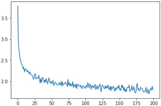
图5.23: RNN 生成器的损失函数

测试

print(evaluate('Th', 200, temperature=0.8))
输出：
Ther
you go what loved ancut that me to the werefered all your to they
That the pessce, shap treed for time sok theie chator
The vuent tere my treance her will not youe
Which my bessin, shall brie lans