R语言模拟：Cross Validation

作者:量化小白一枚，上财研究生在读，偏向数据分析与量化投资

个人公众号:量化小白上分记 

前两篇R语言模拟：Bias Variance Trade-Off与R语言模拟:Bias Variance Decomposition在理论推导和模拟的基础上，对于误差分析中的偏差方差进行了分析。本文在前文的基础上，分析一种常用的估计预测误差进而可以参数优化的方法：交叉验证，并通过R语言进行模拟。

K-FOLD CV

交叉验证是数据建模中一种常用方法，通过交叉验证估计预测误差并有效避免过拟合现象。简要说明CV(CROSS VALIDATION)的逻辑，最常用的是K-FOLD CV，以K = 5为例。

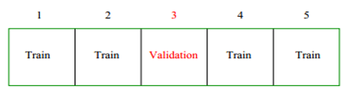
将整个样本集分为K份，每次取其中一份作为Validation Set，剩余四份为Trainset，用Trainset训练模型，然后计算模型在Validation set上的误差，循环k次得到k个误差后求平均，作为预测误差的估计量。

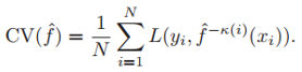
除此之外，比较常用的还有LOOCV，每次只留出一项做Validation，剩余项做Trainset。

参数优化

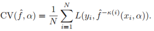
对于含有参数的模型，可以分析模型在不同参数值下的CV的误差，选取误差最小的参数值。

误区

ESL 7.10.2中提到应用CV的两种方法，比如对于一个包含多个自变量的分类模型，建模中包括两方面，一个是筛选出预测能力强的变量，一个是估计最佳的参数。因此有两种使用CV的方法（以下内容摘自ESL 7.10.2）

1

1.Screen the predictors: find a subset of “good” predictors that show fairly strong (univariate) correlation with the class labels

2.Using just this subset of predictors, build a multivariate classifier.

3.Use cross-validation to estimate the unknown tuning parameters and to estimate the prediction error of the final model.

2

1. Divide the samples into K CV folds(group) at random.

2. For each fold k = 1,2,...,K

(a) Find a subset of "good" predictors that show fairly strong  correlation with the class labels, using all of the samples except those in fold k.

(b) Using just this subset of predictors,build a multivariate classifier,using all of the samples except those in fold K.

(c) Use the classifier to predict rhe class labels for the samples in fold k.

简单来说，第一种方法是先使用全样本筛出预测能力强的变量，仅使用这部分变量进行建模，然后用这部分变量建立的模型通过CV优化参数；第二种方法是对全样本CV后，在CV过程中进行筛选变量，然后用筛选出来的变量优化参数，这样CV中每个循环里得到的预测能力强的变量有可能是不一样的。

我们经常使用的是第一种方法，但事实上第一种方法是错误的，直接通过全样本得到的预测能力强的变量，再进行CV，计算出来的误差一定是偏低的。因为筛选过程使用了全样本，再使用CV，用其中K-1份预测1份，使用的预测能力强的变量中实际上包含了这一份的信息，因此存在前视误差。

（The problem is that the predictors have an unfair advantage, as they were chosen in step (1) on the basis of all of the samples. Leaving samples out after the variables have been selected does not correctly mimic the application of the classifier to a completely independent test set, since these predictors “have already seen” the left out samples.）

作者给出一个可以验证的例子：

考虑包含50个样本的二分类集合，两种类别的样本数相同，5000个服从标准正态分布的自变量且均与类别标签独立。这种情况下，理论上使用任何模型得到的误差都应该是50%。 

如果此时我们使用上述方法1找出100个与类别标签相关性最强的变量，然后仅对这100个变量使用KNN算法，并令K=1,CV得到的误差仅有3%，远远低于真实误差50%。

作者使用了5-FOLD CV并且计算了CV中每次Validation set 中10个样本的自变量与类别的相关系数，发现此时相关系数平均值为0.28，远大于0。

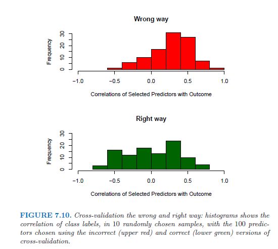
而使用第二种方法计算的相关系数远低于第一种方法。

模拟

 我们通过R语言模拟给出一个通过CV估计最优参数的例子，例子为上一篇右下图的延伸。

样本： 80个样本，20个自变量，自变量均服从[0,1]均匀分布，因变量定义为：

Y = ifelse(X1+X2+...+X10>5,1,0)

使用Best Subset Regression建模（就是在线性回归的基础上加一步筛选最优自变量组合），模型唯一待定参数为Subset Size p，即最优的自变量个数。

通过10-Fold CV计算不同参数p下的预测误差并给出最优的p值，Best Subset Regression可以通过函数regsubsets实现，最终结果如下：

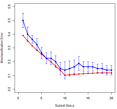
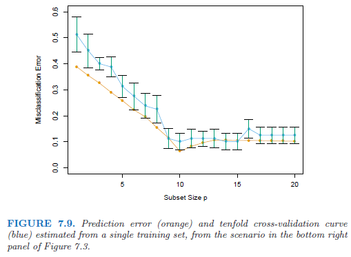
对比教材中的结果

其中，红色线为真实的预测误差，蓝色线为10-FOLD CV计算出的误差，bar为1标准误。可以得出以下结论：

1. CV估计的误差与实际预测误差的数值大小、趋势变化基本相同，并且真实预测误差基本都在CV1标准误以内。

2. p = 10附近误差最小，表明参数p应设定为10，这也与样本因变量定义相符。

可以直接运行的R代码

setwd('xxxx')
library(leaps) 
library(DAAG)
library(caret)
lm.BestSubSet<- function(trainset,k){
 lm.sub <- regsubsets(V21~.,trainset,nbest =1,nvmax = 20)
 summary(lm.sub)
 coef_lm <- coef(lm.sub,k)
 strings_coef_lm <- coef_lm
 x <- paste(names(coef_lm)[2:length(coef_lm)], collapse ='+')
 formulas <- as.formula(paste('V21~',x,collapse=''))
 return(formulas)
}

# ====================   get error ===============================
getError <- function(k,num,modeltype,seeds,n_test){
 set.seed(seeds)
 testset <- as.data.frame(matrix(runif(n_test*21,0,1),n_test))
 
 Allfx_hat <- matrix(0,n_test,num)
 Ally <- matrix(0,n_test,num)
 Allfx <- matrix(0,n_test,num)
  
 # 模拟 num次   
 for (i in 1:num){
   trainset <- as.data.frame(matrix(runif(80*21,0,1),80))
   fx_train <- ifelse(trainset[,1] +trainset[,2] +trainset[,3] +trainset[,4] +trainset[,5]+
                        trainset[,6] +trainset[,7] +trainset[,8] +trainset[,9] +trainset[,10]>5,1,0)   
   trainset[,21] <- fx_train   
   fx_test <- ifelse(testset[,1] +testset[,2] +testset[,3] +testset[,4] +testset[,5]+
                       testset[,6] +testset[,7] +testset[,8] +testset[,9] +testset[,10]>5,1,0)
   
   testset[,21] <- fx_test 
   
   
   # best subset
   lm.sub <- lm(formula = lm.BestSubSet(trainset,k),trainset)
   probs <- predict(lm.sub,testset[,1:20], type = 'response')
   
   
   Allfx_hat[,i] <- probs
   Ally[,i] <- testset[,21]
   Allfx[,i] <- fx_test
   
 } 
 # 计算方差、偏差等
 
 # irreducible <- sigma^2
 
 irreducible  <- mean(apply( Allfx - Ally  ,1,var))
 SquareBais  <- mean(apply((Allfx_hat - Allfx)^2,1,mean))
 Variance <- mean(apply(Allfx_hat,1,var))
 
 # 回归或分类两种情况
 if (modeltype == 'reg'){
   PredictError <- irreducible + SquareBais + Variance 
 }else{
   PredictError <- mean(ifelse(Allfx_hat>=0.5,1,0)!=Allfx)
 }
 result <- data.frame(k,irreducible,SquareBais,Variance,PredictError)
 return(result)
}


# -------------------- classification -------------------
modeltype <- 'classification'
num <- 100
n_test <- 1000
seeds <- 4

all_p <- seq(2,20,1)
result <- getError(1,num,modeltype,seeds,n_test)
for (i in all_p){
 result <- rbind(result,getError(i,num,modeltype,seeds,n_test)) 
}

# ==================== CV  =========================

fun_cv <- function(trainset,kfold=10,seed_num =3,p){
 set.seed(seed_num)
 folds<-createFolds(y=trainset$V21,kfold) 
 misrate <- NULL
 
 for (i in(1:kfold)){
   
   train_cv<-trainset[-folds[[i]],]
   test_cv<-trainset[folds[[i]],]
   
   model <- lm(formula = lm.BestSubSet(train_cv,p),train_cv)
   result  <- predict(model,type='response',test_cv)
   
   # result 
   misrate[i] <- mean( ifelse(result>=0.5,1,0) != test_cv$V21)
 }
 sderror <- sd(misrate)/(length(misrate)^0.5)
 misrate <- mean(misrate)
 result <- data.frame(p,misrate,sderror)
 return(result) 
}

plot_error <- function(x, y, sd, len = 1, col = "black") {
 len <- len * 0.05
 arrows(x0 = x, y0 = y, x1 = x, y1 = y - sd, col = col, angle = 90, length = len)
 arrows(x0 = x, y0 = y, x1 = x, y1 = y + sd, col = col, angle = 90, length = len)
}


# ================================   draw ==============================
# seed =   9,10,   92,65，114,  10912
seed_num =  9
trainset <- as.data.frame(matrix(runif(80*21,0,1),80))
trainset[,21] <- ifelse(trainset[,1] +trainset[,2] +trainset[,3] +trainset[,4] +trainset[,5]+
                         trainset[,6] +trainset[,7] +trainset[,8] +trainset[,9] +trainset[,10]>5,1,0)

resultcv <- fun_cv(trainset,kfold = 10,seed_num,p = 1)
for (p in 2:20){
 resultcv <- rbind(resultcv,fun_cv(trainset,kfold = 10,seed_num,p))
}

png(file = "Cross Validation_large_testset.png")

plot(result$k,result$PredictError,type = 'o',col = 'red',
    xlim = c(0,20),ylim = c(0,0.6),xlab = '', ylab ='', lwd = 2)
par(new = T)

plot(resultcv$p,resultcv$misrate,type='o',lwd=2,col='blue',ylim = c(0,0.6),xlim = c(0,20),
    xlab = 'Subset Size p', ylab = 'Misclassification Error')
plot_error(resultcv$p,resultcv$misrate,resultcv$sderror,col = 'blue',len = 1)
dev.off()

参考文献

Ruppert D. The Elements of Statistical Learning: Data Mining, Inference, and Prediction[J]. Journal of the Royal Statistical Society, 2010, 99(466):567-567.

公众号后台回复关键字即可学习

回复 爬虫            爬虫三大案例实战  
回复 Python       1小时破冰入门

回复 数据挖掘     R语言入门及数据挖掘
回复 人工智能     三个月入门人工智能
回复 数据分析师  数据分析师成长之路 
回复 机器学习      机器学习的商业应用
回复 数据科学      数据科学实战
回复 常用算法      常用数据挖掘算法