Focal Loss和它背后的男人RetinaNet

加入极市专业CV交流群，与 10000+来自港科大、北大、清华、中科院、CMU、腾讯、百度 等名校名企视觉开发者互动交流！

同时提供每月大咖直播分享、真实项目需求对接、干货资讯汇总，行业技术交流。关注 极市平台 公众号 ，回复 加群，立刻申请入群~

说起Focal Loss，相信做CV的都不会陌生，当面临正负样本不平衡时可能第一个想到的就是用Focal Loss试试。但是怕是很多人会不知道这篇论文中所提出的one stage目标检测模型RetinaNet，这也难怪，就连论文里面也说了RetinaNet模型层面没有大的创新，模型效果主要靠Focal Loss。RetinaNet作为RCNN系中one stage检测模型的代表，我觉得依然有学习研究的价值，这不仅会让你加深对RCNN系模型的理解，而且有利于学习后面新的模型，毕竟后面很多模型都是借鉴了RetinaNet。这里将介绍Focal Loss和RetinaNet（比如FCOS和YOLACT），也会给出一些具体的代码实现。

Focal Loss

类别不平衡（class imbalance）是目标检测模型训练的一大难点（推荐这篇综述文章Imbalance Problems in Object Detection: A Review，其中最严重的是正负样本不平衡，因为一张图像的物体一般较少，而目前大部分的目标检测模型在FCN上每个位置密集抽样，无论是基于anchor的方法还是anchor free方法都如此。对于Faster R-CNN这种two stage模型，第一阶段的RPN可以过滤掉很大一部分负样本，最终第二阶段的检测模块只需要处理少量的候选框，而且检测模块还采用正负样本固定比例抽样（比如1:3）或者OHEM方法（online hard example mining）来进一步解决正负样本不平衡问题。对于one stage方法来说，detection部分要直接处理大量的候选位置，其中负样本要占据绝大部分，SSD的策略是采用hard mining，从大量的负样本中选出loss最大的topk的负样本以保证正负样本比例为1:3。其实RPN本质上也是one stage检测模型，RPN训练时所采取的策略也是抽样，从一张图像中抽取固定数量N（RPN采用的是256）的样本，正负样本分开来随机抽样N/2，如果正样本不足，那就用负样本填充，实现代码非常简单：

def subsample_labels(labels, num_samples, positive_fraction, bg_label):    """    Return `num_samples` (or fewer, if not enough found)    random samples from `labels` which is a mixture of positives & negatives.    It will try to return as many positives as possible without    exceeding `positive_fraction * num_samples`, and then try to    fill the remaining slots with negatives.    Args:        labels (Tensor): (N, ) label vector with values:            * -1: ignore            * bg_label: background ("negative") class            * otherwise: one or more foreground ("positive") classes        num_samples (int): The total number of labels with value >= 0 to return.            Values that are not sampled will be filled with -1 (ignore).        positive_fraction (float): The number of subsampled labels with values > 0            is `min(num_positives, int(positive_fraction * num_samples))`. The number            of negatives sampled is `min(num_negatives, num_samples - num_positives_sampled)`.            In order words, if there are not enough positives, the sample is filled with            negatives. If there are also not enough negatives, then as many elements are            sampled as is possible.        bg_label (int): label index of background ("negative") class.    Returns:        pos_idx, neg_idx (Tensor):            1D vector of indices. The total length of both is `num_samples` or fewer.    """    positive = torch.nonzero((labels != -1) & (labels != bg_label), as_tuple=True)[0]    negative = torch.nonzero(labels == bg_label, as_tuple=True)[0]
    num_pos = int(num_samples * positive_fraction)    # protect against not enough positive examples    num_pos = min(positive.numel(), num_pos)    num_neg = num_samples - num_pos    # protect against not enough negative examples    num_neg = min(negative.numel(), num_neg)
    # randomly select positive and negative examples    perm1 = torch.randperm(positive.numel(), device=positive.device)[:num_pos]    perm2 = torch.randperm(negative.numel(), device=negative.device)[:num_neg]
    pos_idx = positive[perm1]    neg_idx = negative[perm2]    return pos_idx, neg_idx

与抽样方法不同，Focal Loss从另外的视角来解决样本不平衡问题，那就是根据置信度动态调整交叉熵loss，当预测正确的置信度增加时，loss的权重系数会逐渐衰减至0，这样模型训练的loss更关注难例，而大量容易的例子其loss贡献很低。这里以二分类来介绍Focal Loss（FL），对二分类最常用的是cross entropy （CE）loss，定义如下：

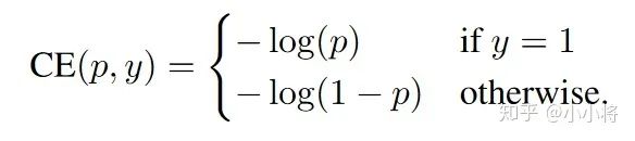
其中 为真实标签，1表示为正例，-1表示为负例；而 为模型预测为正例的概率值。进一步可以定义：

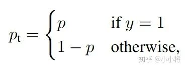
这样CE就可以简写为：

一般情形下，还可以为正例设置权重系数 ，负例权重系数为 ，此时的loss就变为：

如图1所示，蓝色的曲线表示CE，如果定义 的样本的容易例子，从曲线可以看到，这部分简单例子的loss值依然不低，而且这部分例子要占很大比例，加起来后将淹没难例的loss。这就是CE loss用于目标检测模型训练所存在的问题。

图1 FL和CE的对比

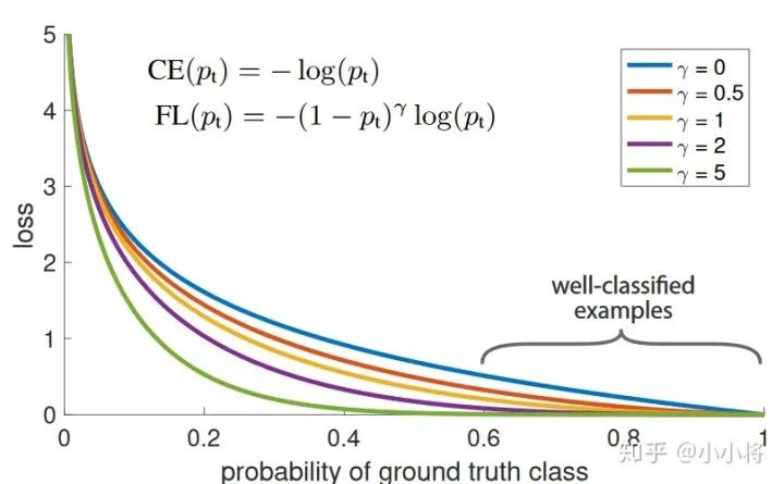
为了解决CE的问题，FL在CE基础上增加一个调节因子 ，FL定义如下：

图1给出了 时的FL曲线，可以看到当 很小时，此时样本被分类，调节因子值接近1，loss不受影响，而当 趋近于1时，调节因子接近0，这样已经能正确分类的简单样例loss大大降低。超参数 为0时，FL等价于CE，论文中发现取2时是最好的，此时若一个样本的 为0.9，其对应的CE loss是FL的100倍，可见FL相比CE可以大大降低简单例子的loss，使模型训练更关注于难例。如果加上类别权重系数，FL变为：

FL的实现也非常简单，这里给出Facebook的官方实现：

def sigmoid_focal_loss(    inputs: torch.Tensor,    targets: torch.Tensor,    alpha: float = -1,    gamma: float = 2,    reduction: str = "none",) -> torch.Tensor:    """    Loss used in RetinaNet for dense detection: https://arxiv.org/abs/1708.02002.    Args:        inputs: A float tensor of arbitrary shape.                The predictions for each example.        targets: A float tensor with the same shape as inputs. Stores the binary                 classification label for each element in inputs                (0 for the negative class and 1 for the positive class).        alpha: (optional) Weighting factor in range (0,1) to balance                positive vs negative examples. Default = -1 (no weighting).        gamma: Exponent of the modulating factor (1 - p_t) to               balance easy vs hard examples.        reduction: 'none' | 'mean' | 'sum'                 'none': No reduction will be applied to the output.                 'mean': The output will be averaged.                 'sum': The output will be summed.    Returns:        Loss tensor with the reduction option applied.    """    p = torch.sigmoid(inputs)    ce_loss = F.binary_cross_entropy_with_logits(inputs, targets, reduction="none")    p_t = p * targets + (1 - p) * (1 - targets)    loss = ce_loss * ((1 - p_t) ** gamma)
    if alpha >= 0:        alpha_t = alpha * targets + (1 - alpha) * (1 - targets)        loss = alpha_t * loss
    if reduction == "mean":        loss = loss.mean()    elif reduction == "sum":        loss = loss.sum()
    return loss

RetinaNet

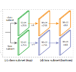
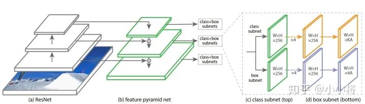
RetinaNet可以看成RPN的多分类升级版，和RPN一样，RetinaNet的backbone也是采用FPN，anchor机制也是类似的，毕竟都属于RCNN系列作品。RetinaNet的整体架构如图2所示，包括FPN backbone以及detection部分，detection部分包括分类分支和预测框分支。

图2 RetinaNet的整体架构

Backbone

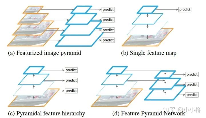
RetinaNet的backbone是基于ResNet的FPN，FPN在原始的CNN基础上增加自上而下的路径和横向连接（lateral connections），如图3d所示。图3a这种是用图像金字塔构建特征金字塔，非常低效；图3b是只取最后的特征；图3c是取CNN的不同层次的特征，SSD是这样的思路，但是FPN更进一步，增加一个自上而下的逻辑，通过横向连接融合不同层次特征。

图3 FPN与其他的类似结构对比

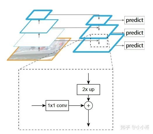
FPN的横向连接如图4所示，高层次特征进行一个2x的上采样（通过简单的最近邻插值实现），然后低层次特征用一个1x1卷积层降维，这样低层次特征和高层次特征维度一致（h, w, c均一致），直接相加。最后跟一个3x3卷积以消除上采样带来的不利影响。

图4 FPN中的横向连接结构

原始的ResNet共有4个stage，其得到的特征分别记为 ，相较于输入图像，它们的stride分别为 。FPN的构建从 开始，首先采用一个1x1卷积得到channel为C（FPN中取256，FPN中所有level的channel都是一样的）的新特征，然后就可以自上而下生成不同level的新特征，分别记为 ，与ResNet的特征是一一对应的，另外对 直接采用一个stride=2的下采样得到一个新特征 （基于stride=2的1x1 maxpooling实现），这样最后FPN实际上得到了5个不同level的特征，其stride分别为 ，特征维度均为C。Faster R-CNN是采用这样的FPN结构，但是RetinaNet却有稍许变动，第一点是只用ResNet的 ，这样通过FPN得到的特征是 ，相当于去掉了 ， 的stride是4，特征很大，去掉它可以减少计算量，后面会讲到RetinaNet的anchor量和detection head都是比RPN更heavy的，这很有必要。另外新增两个特征 和 ， 在 上加一个stride=2的3x3卷积得到， 是在 后面加ReLU和一个stride=2的3x3卷积得到。这样RetinaNet的backbone得到特征也是5个level，分别为 ，其stride分别为 。一点题外话就是FCOS的backbone也是取 ，也算是借鉴了RetinaNet。而YOLOV3的backbone是基于DarkNet-53的FPN，其特征共提取了3个层次，stride分别是 。

Anchor

RetinaNet的anchor和RPN是类似的，RPN的输入特征是 ，每个level的特征每个位置只放置一种scale的anchor，分别为 ，但是却设置3中长宽比 。RetinaNet的输入特征是 ，anchor的设置与RPN一样，但是每个位置增加3个不同的anchor大小 ，这样每个位置共有A=9个anchor，所有level中anchor size的最小值是32，最大值是813。在训练过程中，RetinaNet与RPN采用同样的anchor匹配策略，即一种基于IoU的双阈值策略：计算anchor与所有GT的IoU，取IoU最大值，若大于 ，则认为此anchor为正样本，且负责预测IoU最大的那个GT；若低于 ，则认为此anchor为负样本；若IoU值在 之间，则忽略不参与训练。这样每个GT可能与多个anchor匹配，但可能某个GT与所有anchor的IoU最大值小于 ，尽管不满足阈值条件，此时也应该保证这个GT被IoU值最大的anchor匹配。RPN中设定的两个阈值为 ，而RetinaNet设定的阈值为 。实现代码如下：

# compute IoUs between GT and anchors [M, N]match_quality_matrix = pairwise_iou(targets_per_image.gt_boxes, anchors_per_image)
BELOW_LOW_THRESHOLD = -1BETWEEN_THRESHOLDS = -2low_threshold = 0.4high_threshold = 0.5
# match_quality_matrix is M (gt) x N (predicted)# Max over gt elements (dim 0) to find best gt candidate for each predictionmatched_vals, matches = match_quality_matrix.max(dim=0)
all_matches = matches.clone() # for allow_low_quality_matches
# Assign candidate matches with low quality to negative (unassigned) valuesbelow_low_threshold = matched_vals < low_thresholdbetween_thresholds = (matched_vals >= low_threshold) & (matched_vals < high_threshold)matches[below_low_threshold] = BELOW_LOW_THRESHOLDmatches[between_thresholds] = BETWEEN_THRESHOLDS
# For each gt, find the prediction with which it has highest qualityhighest_quality_foreach_gt, _ = match_quality_matrix.max(dim=1)# Find highest quality match available, even if it is low, including tiesgt_pred_pairs_of_highest_quality = torch.nonzero(            match_quality_matrix == highest_quality_foreach_gt[:, None]        )
pred_inds_to_update = gt_pred_pairs_of_highest_quality[:, 1]matches[pred_inds_to_update] = all_matches[pred_inds_to_update]

匹配的结果就是得到N维度（anchor数量）matches，其值表示与每个anchor匹配的GT index，计算loss时就可以找到对应的label和box，若值为-1，则是负样本，若值为-2，则是需要忽略。

另外，anchors和GT boxes之间的编解码方案与Faster R-CNN完全一样。

detection模块

检测模块主要包括分类分支和box回归分支，其中分类分支用来预测每个位置的各个anchor（数量为 ）的类别概率（类别数为 ），而box回归分支用来预测每个位置各个anchor和GT之间的offset。分类分支包括4个3x3的卷积（ReLU激活函数，channel是256），最后是一个3x3的卷积，输出channel为 ，最后sigmoid激活就可以得到各个anchor预测每个类别的概率，对于RetinaNet来说，每个位置相当于 个二分类问题。box回归分支与分类分支类似，只不过最后输出channel是 ，这也表明RetinaNet的box回归是类别无关的。detection模块在FPN各个level的特征是参数共享的，这点和RPN类似，但是RetinaNet的detection模块是多分类的，而且更deeper。

模型初始化

对于backbone，当然采用的是在ImageNet上预训练的ResNet，其它新增的卷积层就普通初始化。一个额外要注意的点是分类分支最后的卷积层的偏值 初始化为：

这个 相当于是为模型训练开始时每个anchor预测为正例设置一个先验概率值，论文中采用的是0.01，只用这一条策略，基于ResNet50的RetinaNet在COCO上的AP值就能达到30.2。这是因为很多anchor是负例，设置先验值可以大大降低负样本在开始训练时的loss，这样训练更容易，RetinaNet很容易loss出现nan。另外这个策略也在另外一篇论文Is Sampling Heuristics Necessary in Training Deep Object Detectors?中被详细研究，经过少许的改进不需要sampling，也不需要focal loss也可以训练出较好的RetinaNet。

模型训练与预测

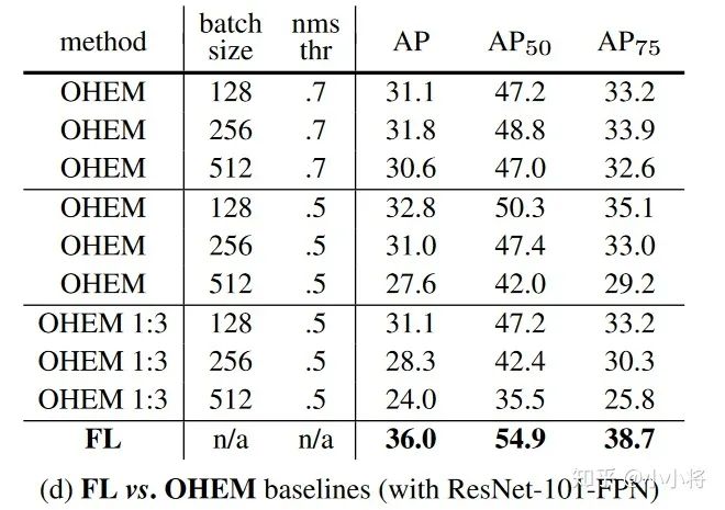
与Faster R-CNN一样，RetinaNet的box回归loss采用smooth L1，但是分类loss采用focal loss，论文中最优参数是 。分类loss是sum所有的focal loss，然后除以类别为正例的anchors总数。论文中FL也和OHEM或者SSD中的OHEM 1:3做了实验对比，发现采用FL的模型训练效果更好：

在inference阶段，对各个level的预测首先取top 1K的detections，然后用0.05的阈值过滤掉负类，此时得到的detections已经大大降低，此时再对detections的box进行解码而不是对模型预测所有detections解码可以提升推理速度。最后把level的detections结果concat在一起，通过IoU=0.5的NMS过滤重叠框就得到最终结果，代码如下：

     boxes_all = []        scores_all = []        class_idxs_all = []
        # Iterate over every feature level        for box_cls_i, box_reg_i, anchors_i in zip(box_cls, box_delta, anchors):            # (HxWxAxK,)            box_cls_i = box_cls_i.flatten().sigmoid_()
            # Keep top k top scoring indices only.            num_topk = min(self.topk_candidates, box_reg_i.size(0))            # torch.sort is actually faster than .topk (at least on GPUs)            predicted_prob, topk_idxs = box_cls_i.sort(descending=True)            predicted_prob = predicted_prob[:num_topk]            topk_idxs = topk_idxs[:num_topk]
            # filter out the proposals with low confidence score            keep_idxs = predicted_prob > self.score_threshold            predicted_prob = predicted_prob[keep_idxs]            topk_idxs = topk_idxs[keep_idxs]
            anchor_idxs = topk_idxs // self.num_classes            classes_idxs = topk_idxs % self.num_classes
            box_reg_i = box_reg_i[anchor_idxs]            anchors_i = anchors_i[anchor_idxs]            # predict boxes            predicted_boxes = self.box2box_transform.apply_deltas(box_reg_i, anchors_i.tensor)
            boxes_all.append(predicted_boxes)            scores_all.append(predicted_prob)            class_idxs_all.append(classes_idxs)
        boxes_all, scores_all, class_idxs_all = [            cat(x) for x in [boxes_all, scores_all, class_idxs_all]        ]        keep = batched_nms(boxes_all, scores_all, class_idxs_all, self.nms_threshold)        keep = keep[: self.max_detections_per_image]
        result = Instances(image_size)        result.pred_boxes = Boxes(boxes_all[keep])        result.scores = scores_all[keep]        result.pred_classes = class_idxs_all[keep]

这里要注意的是由于采用的 个二分类，某个位置的某个anchor可能最后会输出几个类别不同但是box一样的detections。

与其他模型的对比

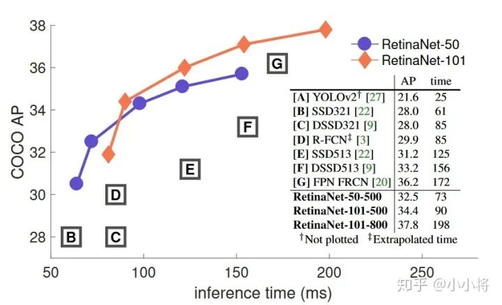
相比SSD和YOLOV2，RetinaNet效果更优，效果对比如下图所示：

最后总结一下RetinaNet与其它同类模型的对比：

• 相比RPN，前面已经说过RetinaNet可以看成RPN的多分类升级版，backbone和FPN设置基本一样，只不过RPN采用简单的sampling方法训练，而RetinaNet采用FL；
• 相比SSD，SSD也是利用多尺度特征，不过RetinaNet是FPN，SSD的anchor与Faster R-CNN类似，不过anchor的size和ratio有稍许差异，另外就是SSD是OHEM 1:3训练，而且采用softmax loss；
• 相比YOLOV3，YOLOv3的backbone是基于DarkNet-53的类FPN结构，level只有3个，不过整体与RetinaNet的backbone接近；YOLOV3的anchor是基于k-means生成，而且匹配策略是基于center和IoU的策略，训练loss是普通的sigmoid。

对比之后，其实发现基于anchor的one stage检测模型差异并没有多大。

参考

1.Focal Loss for Dense Object Detection

2.facebookresearch/detectron2

3.Feature Pyramid Networks for Object Detection

4.Faster R-CNN: Towards Real-Time Object Detection with Region Proposal Networks

5.SSD: Single Shot MultiBox Detector

6.Training Region-based Object Detectors with Online Hard Example Mining

-END -

推荐阅读：

• 深度学习的多个loss如何平衡？

• 人脸识别中Softmax-based Loss的演化史

• 目标检测回归损失函数简介：SmoothL1/IoU/GIoU/DIoU/CIoU Loss

极市独家福利

40万奖金的AI移动应用大赛，参赛就有奖，入围还有额外奖励

添加极市小助手微信 （ID : cv-mart） ，备注： 研究方向-姓名-学校/公司-城市 （如：目标检测-小极-北大-深圳），即可申请加入 目标检测、目标跟踪、人脸、工业检测、医学影像、三维&SLAM、图像分割等极市技术交流群 ，更有 每月大咖直播分享、真实项目需求对接、求职内推、算法竞赛、 干货资讯汇总、行业技术交流 ， 一起来让思想之光照的更远吧~

△长按添加极市小助手

△长按关注极市平台，获取最新CV干货

觉得有用麻烦给个在看啦~