CapsNet入门系列番外:基于TensorFlow实现胶囊网络
编者按:全栈开发者Debarko De简明扼要地介绍了胶囊网络的概念,同时给出了基于numpy和TensorFlow的胶囊网络实现。
什么是胶囊网络?什么是胶囊?胶囊网络比卷积神经网络(CNN)更好吗?本文将讨论这些关于Hinton提出的CapsNet(胶囊网络)的话题。
注意,本文讨论的不是制药学中的胶囊,而是神经网络和机器学习中的胶囊。
阅读本文前,你需要对CNN有基本的了解,否则建议你先看下我之前写的Deep Learning for Noobs。下面我将稍稍温习下与本文相关的CNN的知识,这样你能更容易理解下文CNN与CapsNet的对比。闲话就不多说了,让我们开始吧。
基本上,CNN是堆叠一大堆神经元构成的系统。CNN很擅长处理图像分类问题。让神经网络映射一张图像的所有像素,从算力上来讲,太昂贵了。而卷积在保留数据本质的前提下大大简化了计算。基本上,卷积是一大堆矩阵乘法,再将乘积相加。
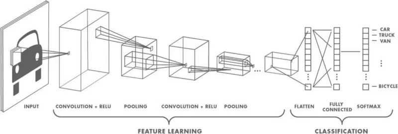
图像传入网络后,一组核或过滤器扫描图像并进行卷积操作,从而创建特征映射。这些特征接着传给之后的激活层和池化层。取决于网络的层数,这一组合可能反复堆叠。激活网络给网络带来了一些非线性(比如ReLU)。池化(比如最大池化)有助于减少训练时间。池化的想法是为每个子区域创建“概要”。同时池化也提供了一些目标检测的位置和平移不变性。网络的最后是一个分类器,比如softmax分类器,分类器返回类别。训练基于对应标注数据的错误进行反向传播。在这一步骤中,非线性有助于解决梯度衰减问题。
CNN有什么问题?
在分类非常接近数据集的图像时,CNN表现极为出色。但CNN在颠倒、倾斜或其他朝向不同的图像上表现很差。训练时添加同一图像的不同变体可以解决这一问题。在CNN中,每层对图像的理解粒度更粗。举个例子,假设你试图分类船和马。最内层(第一层)理解细小的曲线和边缘。第二层可能理解直线或小形状,例如船的桅杆和整个尾巴的曲线。更高层开始理解更复杂的形状,例如整条尾巴或船体。最后层尝试总览全图(例如整条船或整匹马)。我们在每层之后使用池化,以便在合理的时间内完成计算,但本质上池化同时丢失了位置信息。

池化有助于建立位置不变性。否则CNN将只能拟合非常接近训练集的图像或数据。这样的不变性同时导致具备船的部件但顺序错误的图像被误认为船。所以系统会把上图右侧的图像误认为船,而人类则能很清楚地观察到两者的区别。另外,池化也有助于建立比例不变性。

池化本来是用来引入位置、朝向、比例不变性的,然而这一方法非常粗糙。事实上池化加入了各种位置不变性,以致将部件顺序错误的图像也误认为船了。我们需要的不是不变性,而是等价性。不变性使CNN可以容忍视角中的小变动,而等价性使CNN理解朝向和比例变动,并相应地适应图像,从而不损失图像的空间位置信息。CNN会减少自身尺寸以检测较小的船。这导向了最近发展出的胶囊网络。
什么是胶囊网络?
Sara Sabour、Nicholas Frost、Geoffrey Hinton在2017年10月发表了论文Dynamic Routing Between Capsules。当深度学习的祖父之一Geoffrey Hinton发表了一篇论文,这论文注定会是一项重大突破。整个深度学习社区都为此疯狂。这篇论文讨论了胶囊、胶囊网络以及在MNIST上的试验。MNIST是已标注的手写数字图像数据集。相比当前最先进的CNN,胶囊网络在重叠数字上的表现明显提升。论文的作者提出人脑有一个称为“胶囊”的模块,这些胶囊特别擅长处理不同的视觉刺激,以及编码位姿(位置、尺寸、朝向)、变形、速度、反射率、色调、纹理等信息。大脑肯定具备“路由”低层视觉信息至最擅长处理该信息的卷囊的机制。
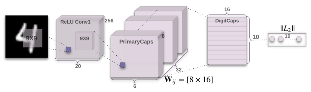
胶囊是一组嵌套的神经网络层。在通常的神经网络中,你不断添加更多层。在胶囊网络中,你会在单个网络层中加入更多的层。换句话说,在一个神经网络层中嵌套另一个。胶囊中的神经元的状态刻画了图像中的一个实体的上述属性。胶囊输出一个表示实体存在性的向量。向量的朝向表示实体的属性。向量发送至神经网络中所有可能的亲本胶囊。胶囊可以为每个可能的亲本计算出一个预测向量,预测向量是通过将自身权重乘以权重矩阵得出的。预测向量乘积标量最大的亲本胶囊的联系将增强,而剩下的亲本胶囊联系将减弱。这一基于合意的路由方法比诸如最大池化之类的现有机制更优越。最大池化路由基于低层网络检测出的最强烈的特征。动态路由之外,胶囊网络给胶囊加上了squash函数。squash属于非线性函数。与CNN给每个网络层添加squash函数不同,胶囊网络给每组嵌套的网络层添加squash函数,从而将squash函数应用到每个胶囊的输出向量。
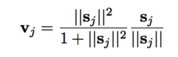
论文引入了一个全新的squash函数(见上图)。ReLU及类似的非线性函数在单个神经元上表现良好,不过论文发现在胶囊上squash函数表现最好。squash函数压缩胶囊的输出向量的长度:当向量较小时,结果为0;当向量较大时,结果为1。动态路由增加了一些额外的运算开销,但毫无疑问带来了优势。
当然我们也要注意,这篇论文刚发不久,胶囊的概念还没有经过全面的测试。它在MNIST数据集上表现良好,但在其他更多种类、更大的数据集上的表现还有待证明。在论文发布的几天之内,就有人提出一些意见。
当前的胶囊网络实现还有改进的空间。不过别忘了Hinton的论文一开始就提到了:
这篇论文的目标不是探索整个空间,而是简单地展示一个相当直接的实现表现良好,同时动态路由有所裨益。
好了,我们已经谈了够多理论了。让我们找点乐子,构建一个胶囊网络。我将引领你阅读一些为MNIST数据配置一个胶囊网络的代码。我会在代码里加上注释,这样你可以逐行理解这些代码是如何工作的。本文将包括两个重要的代码片段。其余代码见GitHub仓库:
     # 只依赖numpy和tensorflow


     import numpy as np


     import tensorflow as tf


     from config import cfg


     # 定义卷积胶囊类,该类由多个神经网络层组成


     #


     class CapsConv(object):


         ''' 胶囊层


         参数:


             input:一个4维张量。


             num_units:整数,胶囊的输出向量的长度。


             with_routing:布尔值,该胶囊路由经过低层胶囊。


             num_outputs:该层中的胶囊数目。


         返回:


             一个4维张量。


         '''


         def __init__(self, num_units, with_routing=True):


             self.num_units = num_units


             self.with_routing = with_routing


         def __call__(self, input, num_outputs, kernel_size=None, stride=None):


             self.num_outputs = num_outputs


             self.kernel_size = kernel_size


             self.stride = stride


             if not self.with_routing:


                 # 主胶囊(PrimaryCaps)层


                 # 输入: [batch_size, 20, 20, 256]


                 assert input.get_shape() == [cfg.batch_size, 20, 20, 256]


                 capsules = []


                 for i in range(self.num_units):


                     # 每个胶囊i: [batch_size, 6, 6, 32]


                     with tf.variable_scope('ConvUnit_' + str(i)):


                         caps_i = tf.contrib.layers.conv2d(input,


                                                           self.num_outputs,


                                                           self.kernel_size,


                                                           self.stride,


                                                           padding="VALID")


                         caps_i = tf.reshape(caps_i, shape=(cfg.batch_size, -1, 1, 1))


                         capsules.append(caps_i)


                 assert capsules[0].get_shape() == [cfg.batch_size, 1152, 1, 1]


                 # [batch_size, 1152, 8, 1]


                 capsules = tf.concat(capsules, axis=2)


                 capsules = squash(capsules)


                 assert capsules.get_shape() == [cfg.batch_size, 1152, 8, 1]


             else:


                 # 数字胶囊(DigitCaps)层


                 # reshape输入至:[batch_size, 1152, 8, 1]


                 self.input = tf.reshape(input, shape=(cfg.batch_size, 1152, 8, 1))


                 # b_IJ: [1, num_caps_l, num_caps_l_plus_1, 1]


                 b_IJ = tf.zeros(shape=[1, 1152, 10, 1], dtype=np.float32)


                 capsules = []


                 for j in range(self.num_outputs):


                     with tf.variable_scope('caps_' + str(j)):


                         caps_j, b_IJ = capsule(input, b_IJ, j)


                         capsules.append(caps_j)


                 # 返回一个张量:[atch_size, 10, 16, 1]


                 capsules = tf.concat(capsules, axis=1)


                 assert capsules.get_shape() == [cfg.batch_size, 10, 16, 1]


             return(capsules)


     def capsule(input, b_IJ, idx_j):


         ''' 层l+1中的单个胶囊的路由算法。


         参数:


             input: 张量 [batch_size, num_caps_l=1152, length(u_i)=8, 1]


                     num_caps_l为l层的胶囊数


         返回:


             张量 [batch_size, 1, length(v_j)=16, 1] 表示


             l+1层的胶囊j的输出向量`v_j`


         注意:


             u_i表示l层胶囊i的输出向量,


             v_j则表示l+1层胶囊j的输出向量


         '''


         with tf.variable_scope('routing'):


             w_initializer = np.random.normal(size=[1, 1152, 8, 16], scale=0.01)


             W_Ij = tf.Variable(w_initializer, dtype=tf.float32)


             # 重复batch_size次W_Ij:[batch_size, 1152, 8, 16]


             W_Ij = tf.tile(W_Ij, [cfg.batch_size, 1, 1, 1])


             # 计算 u_hat


             # [8, 16].T x [8, 1] => [16, 1] => [batch_size, 1152, 16, 1]


             u_hat = tf.matmul(W_Ij, input, transpose_a=True)


             assert u_hat.get_shape() == [cfg.batch_size, 1152, 16, 1]


             shape = b_IJ.get_shape().as_list()


             size_splits = [idx_j, 1, shape[2] - idx_j - 1]


             for r_iter in range(cfg.iter_routing):


                 # 第4行:


                 # [1, 1152, 10, 1]


                 c_IJ = tf.nn.softmax(b_IJ, dim=2)


                 assert c_IJ.get_shape() == [1, 1152, 10, 1]


                 # 第5行:


                 # 在第三维使用c_I加权u_hat


                 # 接着在第二维累加,得到[batch_size, 1, 16, 1]


                 b_Il, b_Ij, b_Ir = tf.split(b_IJ, size_splits, axis=2)


                 c_Il, c_Ij, b_Ir = tf.split(c_IJ, size_splits, axis=2)


                 assert c_Ij.get_shape() == [1, 1152, 1, 1]


                 s_j = tf.multiply(c_Ij, u_hat)


                 s_j = tf.reduce_sum(tf.multiply(c_Ij, u_hat),


                                     axis=1, keep_dims=True)


                 assert s_j.get_shape() == [cfg.batch_size, 1, 16, 1]


                 # 第六行:


                 # 使用上文提及的squash函数,得到:[batch_size, 1, 16, 1]


                 v_j = squash(s_j)


                 assert s_j.get_shape() == [cfg.batch_size, 1, 16, 1]


                 # 第7行:


                 # 平铺v_j,由[batch_size ,1, 16, 1] 至[batch_size, 1152, 16, 1]


                 # [16, 1].T x [16, 1] => [1, 1]


                 # 接着在batch_size维度递归运算均值,得到 [1, 1152, 1, 1]


                 v_j_tiled = tf.tile(v_j, [1, 1152, 1, 1])


                 u_produce_v = tf.matmul(u_hat, v_j_tiled, transpose_a=True)


                 assert u_produce_v.get_shape() == [cfg.batch_size, 1152, 1, 1]


                 b_Ij += tf.reduce_sum(u_produce_v, axis=0, keep_dims=True)


                 b_IJ = tf.concat([b_Il, b_Ij, b_Ir], axis=2)


             return(v_j, b_IJ)


     def squash(vector):


         '''压缩函数


         参数:


             vector:一个4维张量 [batch_size, num_caps, vec_len, 1],


         返回:


             一个和vector形状相同的4维张量,


             但第3维和第4维经过压缩


         '''


         vec_abs = tf.sqrt(tf.reduce_sum(tf.square(vector)))  # 一个标量


         scalar_factor = tf.square(vec_abs) / (1 + tf.square(vec_abs))


         vec_squashed = scalar_factor * tf.divide(vector, vec_abs)  # 对应元素相乘


         return(vec_squashed)
上面是一整个胶囊层。堆叠胶囊层以构成胶囊网络。
     import tensorflow as tf


     from config import cfg


     from utils import get_batch_data


     from capsLayer import CapsConv


     class CapsNet(object):


         def __init__(self, is_training=True):


             self.graph = tf.Graph()


             with self.graph.as_default():


                 if is_training:


                     self.X, self.Y = get_batch_data()


                     self.build_arch()


                     self.loss()


                     # t_vars = tf.trainable_variables()


                     self.optimizer = tf.train.AdamOptimizer()


                     self.global_step = tf.Variable(0, name='global_step', trainable=False)


                     self.train_op = self.optimizer.minimize(self.total_loss, global_step=self.global_step)  # var_list=t_vars)


                 else:


                     self.X = tf.placeholder(tf.float32,


                                             shape=(cfg.batch_size, 28, 28, 1))


                     self.build_arch()


             tf.logging.info('Seting up the main structure')


         def build_arch(self):


             with tf.variable_scope('Conv1_layer'):


                 # Conv1(第一卷积层), [batch_size, 20, 20, 256]


                 conv1 = tf.contrib.layers.conv2d(self.X, num_outputs=256,


                                                  kernel_size=9, stride=1,


                                                  padding='VALID')


                 assert conv1.get_shape() == [cfg.batch_size, 20, 20, 256]


             # TODO: 将'CapsConv'类重写为函数,


             # capsLay函数应该封装为两个函数,


             # 一个类似conv2d,另一个为TensorFlow的fully_connected(全连接)。


             # 主胶囊,[batch_size, 1152, 8, 1]


             with tf.variable_scope('PrimaryCaps_layer'):


                 primaryCaps = CapsConv(num_units=8, with_routing=False)


                 caps1 = primaryCaps(conv1, num_outputs=32, kernel_size=9, stride=2)


                 assert caps1.get_shape() == [cfg.batch_size, 1152, 8, 1]


             # 数字胶囊层,[batch_size, 10, 16, 1]


             with tf.variable_scope('DigitCaps_layer'):


                 digitCaps = CapsConv(num_units=16, with_routing=True)


                 self.caps2 = digitCaps(caps1, num_outputs=10)


             # 前文示意图中的编码器结构


             # 1. 掩码:


             with tf.variable_scope('Masking'):


                 # a). 计算 ||v_c||,接着计算softmax(||v_c||)


                 # [batch_size, 10, 16, 1] => [batch_size, 10, 1, 1]


                 self.v_length = tf.sqrt(tf.reduce_sum(tf.square(self.caps2),


                                                       axis=2, keep_dims=True))


                 self.softmax_v = tf.nn.softmax(self.v_length, dim=1)


                 assert self.softmax_v.get_shape() == [cfg.batch_size, 10, 1, 1]


                 # b). 选取10个胶囊的最大softmax值的索引


                 # [batch_size, 10, 1, 1] => [batch_size] (index)


                 argmax_idx = tf.argmax(self.softmax_v, axis=1, output_type=tf.int32)


                 assert argmax_idx.get_shape() == [cfg.batch_size, 1, 1]


                 # c). 索引


                 # 由于我们是三维生物,


                 # 理解argmax_idx的索引过程并不容易


                 masked_v = []


                 argmax_idx = tf.reshape(argmax_idx, shape=(cfg.batch_size, ))


                 for batch_size in range(cfg.batch_size):


                     v = self.caps2[batch_size][argmax_idx[batch_size], :]


                     masked_v.append(tf.reshape(v, shape=(1, 1, 16, 1)))


                 self.masked_v = tf.concat(masked_v, axis=0)


                 assert self.masked_v.get_shape() == [cfg.batch_size, 1, 16, 1]


             # 2. 使用3个全连接层重建MNIST图像


             # [batch_size, 1, 16, 1] => [batch_size, 16] => [batch_size, 512]


             with tf.variable_scope('Decoder'):


                 vector_j = tf.reshape(self.masked_v, shape=(cfg.batch_size, -1))


                 fc1 = tf.contrib.layers.fully_connected(vector_j, num_outputs=512)


                 assert fc1.get_shape() == [cfg.batch_size, 512]


                 fc2 = tf.contrib.layers.fully_connected(fc1, num_outputs=1024)


                 assert fc2.get_shape() == [cfg.batch_size, 1024]


                 self.decoded = tf.contrib.layers.fully_connected(fc2, num_outputs=784, activation_fn=tf.sigmoid)


         def loss(self):


             # 1. 边际损失


             # [batch_size, 10, 1, 1]


             # max_l = max(0, m_plus-||v_c||)^2


             max_l = tf.square(tf.maximum(0., cfg.m_plus - self.v_length))


             # max_r = max(0, ||v_c||-m_minus)^2


             max_r = tf.square(tf.maximum(0., self.v_length - cfg.m_minus))


             assert max_l.get_shape() == [cfg.batch_size, 10, 1, 1]


             # reshape: [batch_size, 10, 1, 1] => [batch_size, 10]


             max_l = tf.reshape(max_l, shape=(cfg.batch_size, -1))


             max_r = tf.reshape(max_r, shape=(cfg.batch_size, -1))


             # 计算 T_c: [batch_size, 10]


             # T_c = Y,我的理解没错吧?试试看。


             T_c = self.Y


             # [batch_size, 10],对应元素相乘


             L_c = T_c * max_l + cfg.lambda_val * (1 - T_c) * max_r


             self.margin_loss = tf.reduce_mean(tf.reduce_sum(L_c, axis=1))


             # 2. 重建损失


             orgin = tf.reshape(self.X, shape=(cfg.batch_size, -1))


             squared = tf.square(self.decoded - orgin)


             self.reconstruction_err = tf.reduce_mean(squared)


             # 3. 总损失


             self.total_loss = self.margin_loss + 0.0005 * self.reconstruction_err


             # 总结


             tf.summary.scalar('margin_loss', self.margin_loss)


             tf.summary.scalar('reconstruction_loss', self.reconstruction_err)


             tf.summary.scalar('total_loss', self.total_loss)


             recon_img = tf.reshape(self.decoded, shape=(cfg.batch_size, 28, 28, 1))


             tf.summary.image('reconstruction_img', recon_img)


     self.merged_sum = tf.summary.merge_all()
完整代码(含训练和验证模型)见此(https://github.com/debarko/CapsNet-Tensorflow)。代码以Apache 2.0许可发布。我参考了naturomics的代码(https://github.com/naturomics)。
总结
我们介绍了胶囊网络的概念以及如何实现胶囊网络。我们尝试理解胶囊是高层的嵌套神经网络层。我们也查看了胶囊网络是如何交付朝向和其他不变性的——对图像中的每个实体而言,保持空间配置的等价性。我确信存在一些本文没有回答的问题,其中最主要的大概是胶囊及其最佳实现。不过本文是解释这一主题的初步尝试。如果你有任何疑问,请评论。我会尽我所能回答。
Siraj Raval及其演讲对本文影响很大。请在Twitter上分享本文。在twitter关注我以便在未来获取更新信息。
原文地址:https://hackernoon.com/what-is-a-capsnet-or-capsule-network-2bfbe48769cc


