TensorFlow推荐:神经算术逻辑单元的直观理解
编者按:2个月前,DeepMind发表了一篇名为“ 神经算术逻辑单元(NALU)”的新论文,提出了一个能帮助神经网络更好地模拟数值信息的新框架。这是一篇有趣的论文,解决的问题也很实际,所以今天论智想推荐一篇有关这个框架的文章,它也是被TensorFlow官博力荐的佳作。比起复杂的论文解读,它更简洁直观,也易于理解。

现如今,尽管深度学习已经在许多任务中取得了令人惊艳的成果,诸多AI产品也逐渐在医疗等领域发挥越来越重要的作用,但如何教导神经网络还是它的一个重要问题,说出来可能有人不信,神经网络在简单算术任务上还会出现问题。
在一个实验中,DeepMind的研究人员曾训练了一个精度接近完美的模型,它能从数据中找出范围在-5到5之间的数字,但当输入从未见过的新数据后,模型就无法概括了。
论文针对上述问题提出了两种方法,但这里我们不会搬运原文的详细内容,相反地,下文将简要介绍NAC的工作原理,以及它如何处理加减乘除等操作,相应代码也会在文章中列出,读者可以从中获得更直观的了解。
第一个神经网络(NAC)
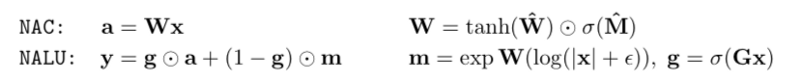
论文介绍的第一个神经网络是神经累积器(简称NAC),它能对输入执行线性变换,而用于变换的矩阵是tanh(What)和sigmoid(Mhat)的元素乘积。简而言之,input(x)后,模型输入会乘以变换矩阵W,并产生输出a。
NAC的Python实现:
     import tensorflow as tf


     # NAC


     W_hat = tf.Variable(tf.truncated_normal(shape, stddev=0.02))


     M_hat = tf.Variable(tf.truncated_normal(shape, stddev=0.02))


     W = tf.tanh(W_hat) * tf.sigmoid(M_hat)


     # 前向传播


     a = tf.matmul(in_dim, W)
第二个神经网络(NALU)
神经算术逻辑单元(NALU)由两个NAC构成,其中,第一个NAC g是sigmoid(Gx),第二个NAC在一个等于exp(W(log(|x| + epsilon)))的对数空间m中运行。
NALU的Python实现:
     import tensorflow as tf


     # NALU


     G = tf.Variable(tf.truncated_normal(shape, stddev=0.02))


     m = tf.exp(tf.matmul(tf.log(tf.abs(in_dim) + epsilon), W))


     g = tf.sigmoid(tf.matmul(in_dim, G))


     y = g * a + (1 - g) * m
通过加法理解NAC
现在我们来进行测试。首先,把NAC转成函数:
     # NAC


     def NAC(in_dim, out_dim):


         in_features = in_dim.shape[1]


         # 定义W_hat和M_hat


         W_hat = tf.get_variable(name = 'W_hat', initializer=tf.initializers.random_uniform(minval=-2, maxval=2),shape=[in_features, out_dim],  trainable=True)


         M_hat = tf.get_variable(name = 'M_hat', initializer=tf.initializers.random_uniform(minval=-2, maxval=2), shape=[in_features, out_dim], trainable=True)


         W = tf.nn.tanh(W_hat) * tf.nn.sigmoid(M_hat)


         a = tf.matmul(in_dim, W)


         return a, W
其次,创建一些数据,把它们分成训练集和测试集。NumPy有一个较numpy.arrange的API,很适合用来创建数据集:
     # 生成一系列输入数字X1和X2用于训练


     x1 = np.arange(0,10000,5, dtype=np.float32)


     x2 = np.arange(5,10005,5, dtype=np.float32)


     y_train = x1 + x2


     x_train = np.column_stack((x1,x2))


     print(x_train.shape)


     print(y_train.shape)


     # 生成一系列输入数字X1和X2进行测试


     x1 = np.arange(1000,2000,8, dtype=np.float32)


     x2 = np.arange(1000,1500,4, dtype= np.float32)


     x_test = np.column_stack((x1,x2))


     y_test = x1 + x2


     print()


     print(x_test.shape)


     print(y_test.shape)
接着,用这些准备好的东西训练模型。我们先定义占位符X和Y以在运行时提供数据,用tf.reduce_sum()计算损失,模型包含两个超参数:学习率alpha和训练几个epochs。在训练开始前,我们还要定义一个优化器,方便用tf.train.AdamOptimizer()降低损失。
     # 定义占位符以在运行时提供输入


     X = tf.placeholder(dtype=tf.float32, shape =[None , 2])    # Number of samples x Number of features (number of inputs to be added)


     Y = tf.placeholder(dtype=tf.float32, shape=[None,])


     #定义网络


     #这里网络只包含一个NAC(用于测试)


     y_pred, W = NAC(in_dim=X, out_dim=1)


     y_pred = tf.squeeze(y_pred)             # Remove extra dimensions if any


     # 均方误差 (MSE)


     loss = tf.reduce_mean( (y_pred - Y) **2)


     # 训练参数


     alpha = 0.05    # learning rate


     epochs = 22000


     optimize = tf.train.AdamOptimizer(learning_rate=alpha).minimize(loss)


     with tf.Session() as sess:


         #init = tf.global_variables_initializer()


         cost_history = []


         sess.run(tf.global_variables_initializer())


         # 训练前损失


         print("Pre training MSE: ", sess.run (loss, feed_dict={X: x_test, Y:y_test}))


         print()


         for i in range(epochs):


             _, cost = sess.run([optimize, loss ], feed_dict={X:x_train, Y: y_train})


             print("epoch: {}, MSE: {}".format( i,cost) )


             cost_history.append(cost)


         # 列出每次迭代的均方误差


         plt.plot(np.arange(epochs),np.log(cost_history))  # Plot MSE on log scale


         plt.xlabel("Epoch")


         plt.ylabel("MSE")


         plt.show()


         print()


         print(W.eval())


         print()


         # 训练后损失


         print("Post training MSE: ", sess.run(loss, feed_dict={X: x_test, Y: y_test}))


         print("Actual sum: ", y_test[0:10])


         print()


         print("Predicted sum: ", sess.run(y_pred[0:10], feed_dict={X: x_test, Y: y_test}))
训练完成后,我们可以得到这样一幅图损失曲线图:
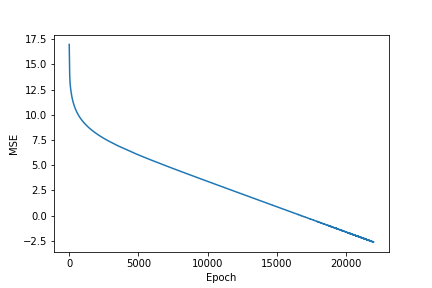
     Actual sum:  [2000. 2012. 2024. 2036. 2048. 2060. 2072. 2084. 2096. 2108.]


     Predicted sum:  [1999.9021 2011.9015 2023.9009 2035.9004 2047.8997 2059.8992 2071.8984


      2083.898  2095.8975 2107.8967]
如输出所示,NAC可以处理诸如加减法的操作,但它还做不到处理乘法和除法。为了解决这个问题,我们就要用到NALU。
通过乘法理解NALU
在上文基础上,首先我们再添加一个NAC,组成NALU:
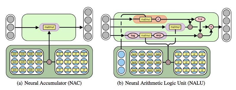
如果说NAC只是对输入做线性变化,那么NALU就是把两个具有权重的NAC组合在一起,用来执行加减(较小的紫色单元)和乘除(较大的紫色单元),计算由门(橙色单元)控制。
     # NALU


     def NALU(in_dim, out_dim):


         shape = (int(in_dim.shape[-1]), out_dim)


         epsilon = 1e-7


         # NAC


         W_hat = tf.Variable(tf.truncated_normal(shape, stddev=0.02))


         M_hat = tf.Variable(tf.truncated_normal(shape, stddev=0.02))


         G = tf.Variable(tf.truncated_normal(shape, stddev=0.02))


         W = tf.tanh(W_hat) * tf.sigmoid(M_hat)


         # 前向传播


         a = tf.matmul(in_dim, W)


         # NALU


         m = tf.exp(tf.matmul(tf.log(tf.abs(in_dim) + epsilon), W))


         g = tf.sigmoid(tf.matmul(in_dim, G))


         y = g * a + (1 - g) * m


         return y
这里我们再创建一些数据,但和上次相比,这次要做一些改动:在第8行和第20行,我们把运算符从加改成了乘。
     # 通过学习乘法来测试网络


     # 生成一系列输入数字X1和X2用于训练


     x1 = np.arange(0,10000,5, dtype=np.float32)


     x2 = np.arange(5,10005,5, dtype=np.float32)


     y_train = x1 * x2


     x_train = np.column_stack((x1,x2))


     print(x_train.shape)


     print(y_train.shape)


     # 生成一系列输入数字X1和X2进行测试


     x1 = np.arange(1000,2000,8, dtype=np.float32)


     x2 = np.arange(1000,1500,4, dtype= np.float32)


     x_test = np.column_stack((x1,x2))


     y_test = x1 * x2


     print()


     print(x_test.shape)


     print(y_test.shape)
之后是训练模型,需要注意的是,这里我们定义的还是NAC,而不是NALU:
     # 定义占位符以在运行时提供值


     X = tf.placeholder(dtype=tf.float32, shape =[None , 2])    # Number of samples x Number of features (number of inputs to be added)


     Y = tf.placeholder(dtype=tf.float32, shape=[None,])


     # 定义网络


     # 这里网络只包含一个NAC(用于测试)


     y_pred = NALU(in_dim=X, out_dim=1)


     y_pred = tf.squeeze(y_pred)      # Remove extra dimensions if any


     # 均方误差 (MSE)


     loss = tf.reduce_mean( (y_pred - Y) **2)


     # 训练参数


     alpha = 0.05    # 学习率


     epochs = 22000


     optimize = tf.train.AdamOptimizer(learning_rate=alpha).minimize(loss)


     with tf.Session() as sess:


         #init = tf.global_variables_initializer()


         cost_history = []


         sess.run(tf.global_variables_initializer())


         # 训练前损失


         print("Pre training MSE: ", sess.run (loss, feed_dict={X: x_test, Y: y_test}))


         print()


         for i in range(epochs):


             _, cost = sess.run([optimize, loss ], feed_dict={X: x_train, Y: y_train})


             print("epoch: {}, MSE: {}".format( i,cost) )


             cost_history.append(cost)


         # 列出每次迭代的损失


         plt.plot(np.arange(epochs),np.log(cost_history))  # Plot MSE on log scale


         plt.xlabel("Epoch")


         plt.ylabel("MSE")


         plt.show()


         # 训练后损失


         print("Post training MSE: ", sess.run(loss, feed_dict={X: x_test, Y: y_test}))


         print("Actual product: ", y_test[0:10])


         print()


         print("Predicted product: ", sess.run(y_pred[0:10], feed_dict={X: x_test, Y: y_test}))
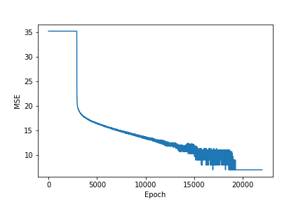
     Actual product:  [1000000. 1012032. 1024128. 1036288. 1048512. 1060800. 1073152. 1085568.


      1098048. 1110592.]


     Predicted product:  [1000000.2  1012032.   1024127.56 1036288.6  1048512.06 1060800.8


      1073151.6  1085567.6  1098047.6  1110592.8 ]
如果想获取在TensorFlow中实现NALU的完整代码,可以去这个github:github.com/ahylton19/simpleNALU-tf
小结
以上只是NALU在加减乘除任务上具体表现,在论文中,研究人员还测试了平方运算和开根,NALU的表现都优于传统框架。简而言之,DeepMind的这个简单而实用的技术让神经网络掌握了数值推算,它类似传统处理器中的算术逻辑单元,能让网络真正“学会”加减乘除和基于加减乘除的近似估计,更好地把经验外推到其他数值任务上,而不再受训练数据限制。
通过这篇文章,我们希望现在你已经了解了这篇轰动学界的论文到底说了什么,以及它对深度学习的贡献和影响。
原文地址:medium.com/tensorflow/understanding-neural-arithmetic-logic-units-11b0f85c1d1d?linkId=57139321