最新翻译的官方 PyTorch 简易入门教程

“PyTorch 深度学习:60分钟快速入门”为 PyTorch 官网教程,网上已经有部分翻译作品,随着PyTorch1.0 版本的公布,这个教程有较大的代码改动,本人对教程进行重新翻译,并测试运行了官方代码,制作成 Jupyter Notebook文件(中文注释)在 github 予以公布。(黄海广)

本文内容较多,可以在线学习,如果需要本地调试,请到github下载:
https://github.com/fengdu78/machine_learning_beginner/tree/master/PyTorch_beginner
此教程为翻译官方地址:
https://pytorch.org/tutorials/beginner/deep_learning_60min_blitz.html
作者: Soumith Chintala
本教程的目标:
在高层次上理解PyTorch的张量(Tensor)库和神经网络
训练一个小型神经网络对图像进行分类
本教程假设您对numpy有基本的了解
注意: 务必确认您已经安装了 torch 和 torchvision 两个包。
目录
一、Pytorch是什么?
二、AUTOGRAD
三、神经网络
四、训练一个分类器
五、数据并行
一、PyTorch 是什么
他是一个基于Python的科学计算包,目标用户有两类
为了使用GPU来替代numpy
一个深度学习研究平台:提供最大的灵活性和速度
开始
张量(Tensors)
张量类似于numpy的ndarrays,不同之处在于张量可以使用GPU来加快计算。
from __future__ import print_function
import torch
构建一个未初始化的5*3的矩阵:
x = torch.Tensor(5, 3)
print(x)
输出 :
tensor([[ 0.0000e+00,  0.0000e+00,  1.3004e-42],
        [ 0.0000e+00,  7.0065e-45,  0.0000e+00],
        [-3.8593e+35,  7.8753e-43,  0.0000e+00],
        [ 0.0000e+00,  1.8368e-40,  0.0000e+00],
        [-3.8197e+35,  7.8753e-43,  0.0000e+00]])
构建一个零矩阵,使用long的类型
      x = torch.zeros(5, 3, dtype=torch.long)
print(x)
输出:
      tensor([[0, 0, 0],
        [0, 0, 0],
        [0, 0, 0],
        [0, 0, 0],
        [0, 0, 0]])
从数据中直接构建一个张量(tensor):
      x = torch.tensor([5.5, 3])
print(x)
输出:
tensor([5.5000, 3.0000])
或者在已有的张量(tensor)中构建一个张量(tensor). 这些方法将重用输入张量(tensor)的属性,例如, dtype,除非用户提供新值
x = x.new_ones(5, 3, dtype=torch.double)      # new_* methods take in sizes
print(x)
x = torch.randn_like(x, dtype=torch.float)    # 覆盖类型!
print(x)                                      # result 的size相同
输出:
tensor([[1., 1., 1.],
        [1., 1., 1.],
        [1., 1., 1.],
        [1., 1., 1.],
        [1., 1., 1.]], dtype=torch.float64)
tensor([[ 1.1701, -0.8342, -0.6769],
        [-1.3060,  0.3636,  0.6758],
        [ 1.9133,  0.3494,  1.1412],
        [ 0.9735, -0.9492, -0.3082],
        [ 0.9469, -0.6815, -1.3808]])
获取张量(tensor)的大小
print(x.size())
输出:
torch.Size([5, 3])
注意
torch.Size实际上是一个元组,所以它支持元组的所有操作。
操作
张量上的操作有多重语法形式,下面我们以加法为例进行讲解。
语法1
y = torch.rand(5, 3)
print(x + y)
输出:
      tensor([[ 1.7199, -0.1819, -0.1543],
        [-0.5413,  1.1591,  1.4098],
        [ 2.0421,  0.5578,  2.0645],
        [ 1.7301, -0.3236,  0.4616],
        [ 1.2805, -0.4026, -0.6916]])
语法二
print(torch.add(x, y))
输出:
      tensor([[ 1.7199, -0.1819, -0.1543],
       [-0.5413,  1.1591,  1.4098],
       [ 2.0421,  0.5578,  2.0645],
       [ 1.7301, -0.3236,  0.4616],
       [ 1.2805, -0.4026, -0.6916]])
语法三:给出一个输出张量作为参数
      result = torch.empty(5, 3)
torch.add(x, y, out=result)
print(result)
输出:
      tensor([[ 1.7199, -0.1819, -0.1543],
       [-0.5413,  1.1591,  1.4098],
       [ 2.0421,  0.5578,  2.0645],
       [ 1.7301, -0.3236,  0.4616],
       [ 1.2805, -0.4026, -0.6916]])
语法四:原地操作(in-place)
# 把x加到y上
y.add_(x)
print(y)
输出:
      tensor([[ 1.7199, -0.1819, -0.1543],
       [-0.5413,  1.1591,  1.4098],
       [ 2.0421,  0.5578,  2.0645],
       [ 1.7301, -0.3236,  0.4616],
       [ 1.2805, -0.4026, -0.6916]])
注意
任何在原地(in-place)改变张量的操作都有一个’_‘后缀。例如x.copy_(y), x.t_()操作将改变x.
你可以使用所有的numpy索引操作。你可以使用各种类似标准NumPy的花哨的索引功能
print(x[:, 1])
输出:
tensor([-0.8342, 0.3636, 0.3494, -0.9492, -0.6815])
调整大小:如果要调整张量/重塑张量,可以使用torch.view:
x = torch.randn(4, 4)
y = x.view(16)
z = x.view(-1, 8)  # -1的意思是没有指定维度
print(x.size(), y.size(), z.size())
输出:
torch.Size([4, 4]) torch.Size([16]) torch.Size([2, 8])
如果你有一个单元素张量,使用.item()将值作为Python数字
x = torch.randn(1)
print(x)
print(x.item())
输出:
tensor([0.3441])
0.34412217140197754
numpy 桥
把一个 torch 张量转换为 numpy 数组或者反过来都是很简单的。
Torch 张量和 numpy 数组将共享潜在的内存,改变其中一个也将改变另一个。
把 Torch 张量转换为 numpy 数组
a = torch.ones(5)
print(a)
输出:
tensor([1., 1., 1., 1., 1.])
输入:
b = a.numpy()
print(b)
print(type(b))
输出:
[ 1.  1.  1.  1.  1.]
<class 'numpy.ndarray'>
通过如下操作,我们看一下numpy数组的值如何在改变。
a.add_(1)
print(a)
print(b)
输出:
tensor([2., 2., 2., 2., 2.])
[ 2.  2.  2.  2.  2.]
把 numpy 数组转换为 torch 张量
看看改变 numpy 数组如何自动改变 torch 张量。
import numpy as np
a = np.ones(5)
b = torch.from_numpy(a)
np.add(a, 1, out=a)
print(a)
print(b)
输出:
[ 2.  2.  2.  2.  2.]
tensor([2., 2., 2., 2., 2.], dtype=torch.float64)
所有在CPU上的张量,除了字符张量,都支持在numpy之间转换。
CUDA 张量
可以使用.to方法将张量移动到任何设备上。
      # let us run this cell only if CUDA is available
# We will use ``torch.device`` objects to move tensors in and out of GPU
if torch.cuda.is_available():
    device = torch.device("cuda")          # a CUDA device object
    y = torch.ones_like(x, device=device)  # directly create a tensor on GPU
    x = x.to(device)                       # or just use strings ``.to("cuda")``
    z = x + y
    print(z)
    print(z.to("cpu", torch.double))       # ``.to`` can also change dtype together!
脚本总运行时间:0.003秒
二、Autograd: 自动求导(automatic differentiation)
PyTorch 中所有神经网络的核心是autograd包.我们首先简单介绍一下这个包,然后训练我们的第一个神经网络.
autograd包为张量上的所有操作提供了自动求导.它是一个运行时定义的框架,这意味着反向传播是根据你的代码如何运行来定义,并且每次迭代可以不同.
接下来我们用一些简单的示例来看这个包:
张量(Tensor)
torch.Tensor是包的核心类。如果将其属性.requires_grad设置为True,则会开始跟踪其上的所有操作。完成计算后,您可以调用.backward()并自动计算所有梯度。此张量的梯度将累积到.grad属性中。
要阻止张量跟踪历史记录,可以调用.detach()将其从计算历史记录中分离出来,并防止将来的计算被跟踪。
要防止跟踪历史记录(和使用内存),您还可以使用torch.no_grad()包装代码块:在评估模型时,这可能特别有用,因为模型可能具有requires_grad = True的可训练参数,但我们不需要梯度。
还有一个类对于autograd实现非常重要 - Function。
Tensor和Function互相连接并构建一个非循环图构建一个完整的计算过程。每个张量都有一个.grad_fn属性,该属性引用已创建Tensor的Function(除了用户创建的Tensors - 它们的grad_fn为None)。
如果要计算导数,可以在Tensor上调用.backward()。如果Tensor是标量(即它包含一个元素数据),则不需要为backward()指定任何参数,但是如果它有更多元素,则需要指定一个梯度参数,该参数是匹配形状的张量。
import torch
创建一个张量并设置requires_grad = True以跟踪它的计算
      x = torch.ones(2, 2, requires_grad=True)
print(x)
输出:
tensor([[1., 1.],
        [1., 1.]], requires_grad=True)
在张量上执行操作:
y = x + 2
print(y)
输出:
tensor([[3., 3.],
        [3., 3.]], grad_fn=<AddBackward>)
因为y是通过一个操作创建的,所以它有grad_fn,而x是由用户创建,所以它的grad_fn为None.
print(y.grad_fn)
print(x.grad_fn)
输出:
<AddBackward object at 0x000001C015ADFFD0>
None
在y上执行操作
z = y * y * 3
out = z.mean()
print(z, out)
输出:
tensor([[27., 27.],
        [27., 27.]], grad_fn=<MulBackward0>) tensor(27., grad_fn=<MeanBackward1>)
.requires_grad_(...)就地更改现有的Tensor的requires_grad标志。 如果没有给出,输入标志默认为False。
a = torch.randn(2, 2)
a = ((a * 3) / (a - 1))
print(a.requires_grad)
a.requires_grad_(True)
print(a.requires_grad)
b = (a * a).sum()
print(b.grad_fn)
输出:
False
True
<SumBackward0 object at 0x000001E020B79FD0>
梯度(Gradients)
现在我们来执行反向传播,out.backward()相当于执行out.backward(torch.tensor(1.))
out.backward()
输出out对x的梯度d(out)/dx:
print(x.grad)
输出:
tensor([[4.5000, 4.5000],
        [4.5000, 4.5000]])
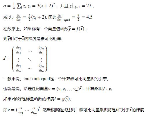
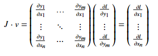
你应该得到一个值全为4.5的矩阵,我们把张量out称为"o". 则:
雅可比向量积的这种特性使得将外部梯度馈送到具有非标量输出的模型中非常方便。
现在让我们来看一个雅可比向量积的例子:
x = torch.randn(3, requires_grad=True)
y = x * 2
while y.data.norm() < 1000:
    y = y * 2
print(y)
输出:
tensor([ 384.5854, -13.6405, -1049.2870], grad_fn=<MulBackward0>)
现在在这种情况下,y不再是标量。 torch.autograd无法直接计算完整雅可比行列式,但如果我们只想要雅可比向量积,只需将向量作为参数向后传递:
v = torch.tensor([0.1, 1.0, 0.0001], dtype=torch.float)
y.backward(v)
print(x.grad)
输出:
tensor([5.1200e+01, 5.1200e+02, 5.1200e-02])
您还可以通过torch.no_grad()代码,在张量上使用.requires_grad = True来停止使用跟踪历史记录。
print(x.requires_grad)
print((x ** 2).requires_grad)
with torch.no_grad():
    print((x ** 2).requires_grad)
输出:
True
True
False
关于 autograd 和 Function 的文档在 http://pytorch.org/docs/autograd
三、神经网络
可以使用 torch.nn 包来构建神经网络.
你已知道 autograd 包,nn 包依赖 autograd 包来定义模型并求导.一个 nn.Module 包含各个层和一个 forward(input) 方法,该方法返回 output.
例如,我们来看一下下面这个分类数字图像的网络.
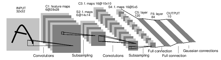
convnet
他是一个简单的前馈神经网络,它接受一个输入,然后一层接着一层的输入,直到最后得到结果.
神经网络的典型训练过程如下:
定义神经网络模型,它有一些可学习的参数(或者权重);
在数据集上迭代;
通过神经网络处理输入;
计算损失(输出结果和正确值的差距大小)
将梯度反向传播会网络的参数;
更新网络的参数,主要使用如下简单的更新原则:
weight = weight - learning_rate * gradient
定义网络
我们先定义一个网络
import torch
import torch.nn as nn
import torch.nn.functional as F

class Net(nn.Module):

    def __init__(self):
        super(Net, self).__init__()
        # 1 input image channel, 6 output channels, 5x5 square convolution
        # kernel
        self.conv1 = nn.Conv2d(1, 6, 5)
        self.conv2 = nn.Conv2d(6, 16, 5)
        # an affine operation: y = Wx + b
        self.fc1 = nn.Linear(16 * 5 * 5, 120)
        self.fc2 = nn.Linear(120, 84)
        self.fc3 = nn.Linear(84, 10)

    def forward(self, x):
        # Max pooling over a (2, 2) window
        x = F.max_pool2d(F.relu(self.conv1(x)), (2, 2))
        # If the size is a square you can only specify a single number
        x = F.max_pool2d(F.relu(self.conv2(x)), 2)
        x = x.view(-1, self.num_flat_features(x))
        x = F.relu(self.fc1(x))
        x = F.relu(self.fc2(x))
        x = self.fc3(x)
        return x

    def num_flat_features(self, x):
        size = x.size()[1:]  # all dimensions except the batch dimension
        num_features = 1
        for s in size:
            num_features *= s
        return num_features


net = Net()
print(net)
输出:
      Net(
  (conv1): Conv2d(1, 6, kernel_size=(5, 5), stride=(1, 1))
  (conv2): Conv2d(6, 16, kernel_size=(5, 5), stride=(1, 1))
  (fc1): Linear(in_features=400, out_features=120, bias=True)
  (fc2): Linear(in_features=120, out_features=84, bias=True)
  (fc3): Linear(in_features=84, out_features=10, bias=True)
)
你只需定义forward函数,backward函数(计算梯度)在使用autograd时自动为你创建.你可以在forward函数中使用Tensor的任何操作.
net.parameters()返回模型需要学习的参数。
      params = list(net.parameters())
print(len(params))
print(params[0].size())
输出:
10
torch.Size([6, 1, 5, 5])f
让我们尝试一个随机的 32x32 输入。 注意:此网络(LeNet)的预期输入大小为 32x32。 要在MNIST数据集上使用此网络,请将数据集中的图像大小调整为 32x32。
input = torch.randn(1, 1, 32, 32)
out = net(input)
print(out)
输出:
      tensor([[-0.1217,  0.0449, -0.0392, -0.1103, -0.0534, -0.1108, -0.0565,  0.0116,
          0.0867,  0.0102]], grad_fn=<AddmmBackward>)
将所有参数的梯度缓存清零,然后进行随机梯度的的反向传播.
net.zero_grad()
out.backward(torch.randn(1, 10))
注意
torch.nn只支持小批量输入,整个torch.nn包都只支持小批量样本,而不支持单个样本例如,nn.Conv2d将接受一个4维的张量,每一维分别是:
nSamples×nChannels×Height×Width(样本数*通道数*高*宽).
如果你有单个样本,只需使用
input.unsqueeze(0)来添加其它的维数.
在继续之前,我们回顾一下到目前为止见过的所有类.
回顾
torch.Tensor-支持自动编程操作(如backward())的多维数组。 同时保持梯度的张量。nn.Module-神经网络模块.封装参数,移动到GPU上运行,导出,加载等nn.Parameter-一种张量,当把它赋值给一个Module时,被自动的注册为参数.autograd.Function-实现一个自动求导操作的前向和反向定义, 每个张量操作都会创建至少一个Function节点,该节点连接到创建张量并对其历史进行编码的函数。
损失函数
一个损失函数接受一对(output, target)作为输入(output为网络的输出,target为实际值),计算一个值来估计网络的输出和目标值相差多少.
在nn包中有几种不同的损失函数.一个简单的损失函数是:nn.MSELoss,他计算输入(个人认为是网络的输出)和目标值之间的均方误差.
例如:
      output = net(input)
target = torch.randn(10)  # a dummy target, for example
target = target.view(1, -1)  # make it the same shape as output
criterion = nn.MSELoss()
loss = criterion(output, target)
print(loss)
输出:
tensor(0.5663, grad_fn=<MseLossBackward>)
现在,你反向跟踪loss,使用它的.grad_fn属性,你会看到向下面这样的一个计算图:
input -> conv2d -> relu -> maxpool2d -> conv2d -> relu -> maxpool2d
      -> view -> linear -> relu -> linear -> relu -> linear
      -> MSELoss
      -> loss
所以, 当你调用loss.backward(),整个图被区分为损失以及图中所有具有requires_grad = True的张量,并且其.grad 张量的梯度累积。
为了说明,我们反向跟踪几步:
print(loss.grad_fn)  # MSELoss
print(loss.grad_fn.next_functions[0][0])  # Linear
print(loss.grad_fn.next_functions[0][0].next_functions[0][0])
输出:
<MseLossBackward object at 0x0000029E54C509B0>
<AddmmBackward object at 0x0000029E54C50898>
<AccumulateGrad object at 0x0000029E54C509B0>
反向传播
为了反向传播误差,我们所需做的是调用loss.backward().你需要清除已存在的梯度,否则梯度将被累加到已存在的梯度。
现在,我们将调用loss.backward(),并查看conv1层的偏置项在反向传播前后的梯度。
net.zero_grad()     # zeroes the gradient buffers of all parameters
print('conv1.bias.grad before backward')
print(net.conv1.bias.grad)
loss.backward()
print('conv1.bias.grad after backward')
print(net.conv1.bias.grad)
输出:
conv1.bias.grad before backward
tensor([0., 0., 0., 0., 0., 0.])
conv1.bias.grad after backward
tensor([ 0.0006, -0.0164,  0.0122, -0.0060, -0.0056, -0.0052])
更新权重
实践中最简单的更新规则是随机梯度下降(SGD)。
weight=weight−learning_rate∗gradient
我们可以使用简单的 Python 代码实现这个规则.
learning_rate = 0.01
for f in net.parameters():
    f.data.sub_(f.grad.data * learning_rate)
然而,当你使用神经网络是,你想要使用各种不同的更新规则,比如SGD,Nesterov-SGD,Adam, RMSPROP等.为了能做到这一点,我们构建了一个包torch.optim实现了所有的这些规则.使用他们非常简单:
import torch.optim as optim
# create your optimizer
optimizer = optim.SGD(net.parameters(), lr=0.01)
# in your training loop:
optimizer.zero_grad()   # zero the gradient buffers
output = net(input)
loss = criterion(output, target)
loss.backward()
optimizer.step()    # Does the update
注意
观察如何使用optimizer.zero_grad()手动将梯度缓冲区设置为零。 这是因为梯度是反向传播部分中的说明那样是累积的。
四、训练一个分类器
你已经学会如何去定义一个神经网络,计算损失值和更新网络的权重。
你现在可能在思考:数据哪里来呢?
关于数据
通常,当你处理图像,文本,音频和视频数据时,你可以使用标准的Python包来加载数据到一个numpy数组中.然后把这个数组转换成torch.*Tensor。
对于图像,有诸如Pillow,OpenCV包等非常实用
对于音频,有诸如scipy和librosa包
对于文本,可以用原始Python和Cython来加载,或者使用NLTK和SpaCy 对于视觉,我们创建了一个
torchvision包,包含常见数据集的数据加载,比如Imagenet,CIFAR10,MNIST等,和图像转换器,也就是torchvision.datasets和torch.utils.data.DataLoader。
这提供了巨大的便利,也避免了代码的重复。
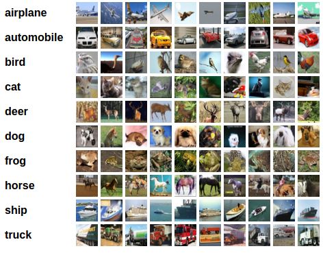
在这个教程中,我们使用CIFAR10数据集,它有如下10个类别:’airplane’,’automobile’,’bird’,’cat’,’deer’,’dog’,’frog’,’horse’,’ship’,’truck’。这个数据集中的图像大小为3*32*32,即,3通道,32*32像素。
在这个教程中,我们使用CIFAR10数据集,它有如下10个类别:’airplane’,’automobile’,’bird’,’cat’,’deer’,’dog’,’frog’,’horse’,’ship’,’truck’.这个数据集中的图像大小为3*32*32,即,3通道,32*32像素.
训练一个图像分类器
我们将按照下列顺序进行:
使用
torchvision加载和归一化CIFAR10训练集和测试集.定义一个卷积神经网络
定义损失函数
在训练集上训练网络
在测试集上测试网络
1. 加载和归一化 CIFAR0
使用 torchvision 加载 CIFAR10 是非常容易的。
import torch
import torchvision
import torchvision.transforms as transforms
torchvision 的输出是 [0,1] 的 PILImage 图像,我们把它转换为归一化范围为 [-1, 1] 的张量。
transform = transforms.Compose(
    [transforms.ToTensor(),
     transforms.Normalize((0.5, 0.5, 0.5), (0.5, 0.5, 0.5))])
trainset = torchvision.datasets.CIFAR10(root='./data', train=True,
                                        download=True, transform=transform)
trainloader = torch.utils.data.DataLoader(trainset, batch_size=4,
                                          shuffle=True, num_workers=2)
testset = torchvision.datasets.CIFAR10(root='./data', train=False,
                                       download=True, transform=transform)
testloader = torch.utils.data.DataLoader(testset, batch_size=4,
                                         shuffle=False, num_workers=2)
classes = ('plane', 'car', 'bird', 'cat',
           'deer', 'dog', 'frog', 'horse', 'ship', 'truck')
#这个过程有点慢,会下载大约340mb图片数据。
torchvision的输出是[0,1]的PILImage图像,我们把它转换为归一化范围为[-1, 1]的张量.
输出:
Files already downloaded and verified
Files already downloaded and verified
我们展示一些有趣的训练图像。
import matplotlib.pyplot as plt
import numpy as np
# functions to show an image
def imshow(img):
    img = img / 2 + 0.5     # unnormalize
    npimg = img.numpy()
    plt.imshow(np.transpose(npimg, (1, 2, 0)))
    plt.show()
# get some random training images
dataiter = iter(trainloader)
images, labels = dataiter.next()

# show images
imshow(torchvision.utils.make_grid(images))
# print labels
print(' '.join('%5s' % classes[labels[j]] for j in range(4)))
输出:

plane deer dog plane
2. 定义一个卷积神经网络
从之前的神经网络一节复制神经网络代码,并修改为接受3通道图像取代之前的接受单通道图像。
import torch.nn as nn
import torch.nn.functional as F

class Net(nn.Module):
    def __init__(self):
        super(Net, self).__init__()
        self.conv1 = nn.Conv2d(3, 6, 5)
        self.pool = nn.MaxPool2d(2, 2)
        self.conv2 = nn.Conv2d(6, 16, 5)
        self.fc1 = nn.Linear(16 * 5 * 5, 120)
        self.fc2 = nn.Linear(120, 84)
        self.fc3 = nn.Linear(84, 10)

    def forward(self, x):
        x = self.pool(F.relu(self.conv1(x)))
        x = self.pool(F.relu(self.conv2(x)))
        x = x.view(-1, 16 * 5 * 5)
        x = F.relu(self.fc1(x))
        x = F.relu(self.fc2(x))
        x = self.fc3(x)
        return x

net = Net()
3. 定义损失函数和优化器
我们使用交叉熵作为损失函数,使用带动量的随机梯度下降。
import torch.optim as optim
criterion = nn.CrossEntropyLoss()
optimizer = optim.SGD(net.parameters(), lr=0.001, momentum=0.9)
4. 训练网络
这是开始有趣的时刻,我们只需在数据迭代器上循环,把数据输入给网络,并优化。
for epoch in range(2):  # loop over the dataset multiple times

    running_loss = 0.0
    for i, data in enumerate(trainloader, 0):
        # get the inputs
        inputs, labels = data
        # zero the parameter gradients
        optimizer.zero_grad()
        # forward + backward + optimize
        outputs = net(inputs)
        loss = criterion(outputs, labels)
        loss.backward()
        optimizer.step()
        # print statistics
        running_loss += loss.item()
        if i % 2000 == 1999:    # print every 2000 mini-batches
            print('[%d, %5d] loss: %.3f' %
                  (epoch + 1, i + 1, running_loss / 2000))
            running_loss = 0.0

print('Finished Training')
输出:
[1,  2000] loss: 2.286
[1,  4000] loss: 1.921
[1,  6000] loss: 1.709
[1,  8000] loss: 1.618
[1, 10000] loss: 1.548
[1, 12000] loss: 1.496
[2,  2000] loss: 1.435
[2,  4000] loss: 1.409
[2,  6000] loss: 1.373
[2,  8000] loss: 1.348
[2, 10000] loss: 1.326
[2, 12000] loss: 1.313
Finished Training
5. 在测试集上测试网络
我们在整个训练集上训练了两次网络,但是我们还需要检查网络是否从数据集中学习到东西。
我们通过预测神经网络输出的类别标签并根据实际情况进行检测,如果预测正确,我们把该样本添加到正确预测列表。
第一步,显示测试集中的图片一遍熟悉图片内容。
dataiter = iter(testloader)
images, labels = dataiter.next()
# print images
imshow(torchvision.utils.make_grid(images))
print('GroundTruth: ', ' '.join('%5s' % classes[labels[j]] for j in range(4)))
输出:
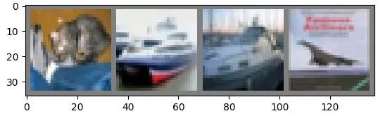
GroundTruth: cat ship ship plane
现在我们来看看神经网络认为以上图片是什么?
outputs = net(images)
输出是10个标签的概率。一个类别的概率越大,神经网络越认为他是这个类别。所以让我们得到最高概率的标签。
_, predicted = torch.max(outputs, 1)
print('Predicted: ', ' '.join('%5s' % classes[predicted[j]]
                              for j in range(4)))
输出:
Predicted: cat ship ship plane
这结果看起来非常的好。
接下来让我们看看网络在整个测试集上的结果如何。
correct = 0
total = 0
with torch.no_grad():
    for data in testloader:
        images, labels = data
        outputs = net(images)
        _, predicted = torch.max(outputs.data, 1)
        total += labels.size(0)
        correct += (predicted == labels).sum().item()

print('Accuracy of the network on the 10000 test images: %d %%' % (
    100 * correct / total))
输出:
Accuracy of the network on the 10000 test images: 54 %
结果看起来好于偶然,偶然的正确率为10%,似乎网络学习到了一些东西。
那在什么类上预测较好,什么类预测结果不好呢?
class_correct = list(0. for i in range(10))
class_total = list(0. for i in range(10))
with torch.no_grad():
    for data in testloader:
        images, labels = data
        outputs = net(images)
        _, predicted = torch.max(outputs, 1)
        c = (predicted == labels).squeeze()
        for i in range(4):
            label = labels[i]
            class_correct[label] += c[i].item()
            class_total[label] += 1
for i in range(10):
    print('Accuracy of %5s : %2d %%' % (
        classes[i], 100 * class_correct[i] / class_total[i]))
输出:
Accuracy of plane : 52 %
Accuracy of   car : 63 %
Accuracy of  bird : 43 %
Accuracy of   cat : 33 %
Accuracy of  deer : 36 %
Accuracy of   dog : 46 %
Accuracy of  frog : 68 %
Accuracy of horse : 62 %
Accuracy of  ship : 80 %
Accuracy of truck : 63 %
在GPU上训练
你是如何把一个 Tensor 转换 GPU 上,你就如何把一个神经网络移动到 GPU 上训练。这个操作会递归遍历有所模块,并将其参数和缓冲区转换为 CUDA 张量。
device = torch.device("cuda:0" if torch.cuda.is_available() else "cpu")
# Assume that we are on a CUDA machine, then this should print a CUDA device:
#假设我们有一台CUDA的机器,这个操作将显示CUDA设备。
print(device)
输出:
cuda:0
接下来假设我们有一台CUDA的机器,然后这些方法将递归遍历所有模块并将其参数和缓冲区转换为CUDA张量:
net.to(device)
输出:
Net(
  (conv1): Conv2d(3, 6, kernel_size=(5, 5), stride=(1, 1))
  (pool): MaxPool2d(kernel_size=2, stride=2, padding=0, dilation=1, ceil_mode=False)
  (conv2): Conv2d(6, 16, kernel_size=(5, 5), stride=(1, 1))
  (fc1): Linear(in_features=400, out_features=120, bias=True)
  (fc2): Linear(in_features=120, out_features=84, bias=True)
  (fc3): Linear(in_features=84, out_features=10, bias=True)
)
请记住,你也必须在每一步中把你的输入和目标值转换到 GPU 上:
inputs, labels = inputs.to(device), labels.to(device)
为什么我们没注意到GPU的速度提升很多?那是因为网络非常的小.
实践:尝试增加你的网络的宽度(第一个nn.Conv2d的第2个参数, 第二个nn.Conv2d的第一个参数,他们需要是相同的数字),看看你得到了什么样的加速。
实现的目标:
深入了解了PyTorch的张量库和神经网络.
训练了一个小网络来分类图片.
五、数据并行(选读)
作者:Sung Kim和Jenny Kang
在这个教程里,我们将学习如何使用数据并行(DataParallel)来使用多GPU。
PyTorch非常容易的就可以使用GPU,你可以用如下方式把一个模型放到GPU上:
device = torch.device("cuda:0")
model.to(device)
然后你可以复制所有的张量到GPU上:
mytensor = my_tensor.to(device)
请注意,只调用mytensor.gpu()并没有复制张量到 GPU 上。你需要把它赋值给一个新的张量并在 GPU 上使用这个张量。
在多 GPU 上执行前向和反向传播是自然而然的事。然而,PyTorch 默认将只是用一个GPU。你可以使用 DataParallel 让模型并行运行来轻易的让你的操作在多个 GPU 上运行。
model = nn.DataParallel(model)
这是这篇教程背后的核心,我们接下来将更详细的介绍它。
导入和参数
导入PyTorch模块和定义参数。
import torch
import torch.nn as nn
from torch.utils.data import Dataset, DataLoader
# Parameters and DataLoaders
input_size = 5
output_size = 2
batch_size = 30
data_size = 100
设备:
device = torch.device("cuda:0" if torch.cuda.is_available() else "cpu")
虚拟数据集
制作一个虚拟(随机)数据集,你只需实现__getitem__。
class RandomDataset(Dataset):
    def __init__(self, size, length):
        self.len = length
        self.data = torch.randn(length, size)
    def __getitem__(self, index):
        return self.data[index]
    def __len__(self):
        return self.len
rand_loader = DataLoader(dataset=RandomDataset(input_size, data_size),
                         batch_size=batch_size, shuffle=True)
简单模型
作为演示,我们的模型只接受一个输入,执行一个线性操作,然后得到结果。然而,你能在任何模型(CNN,RNN,Capsule Net等)上使用DataParallel。
我们在模型内部放置了一条打印语句来检测输入和输出向量的大小。请注意批等级为0时打印的内容。
class Model(nn.Module):
    # Our model
    def __init__(self, input_size, output_size):
        super(Model, self).__init__()
        self.fc = nn.Linear(input_size, output_size)
    def forward(self, input):
        output = self.fc(input)
        print("	In Model: input size", input.size(),
              "output size", output.size())
        return output
创建一个模型和数据并行
这是本教程的核心部分。首先,我们需要创建一个模型实例和检测我们是否有多个 GPU。如果我们有多个 GPU,我们使用 nn.DataParallel 来包装我们的模型。然后通过 model.to(device) 把模型放到 GPU 上。
model = Model(input_size, output_size)
if torch.cuda.device_count() > 1:
  print("Let's use", torch.cuda.device_count(), "GPUs!")
  # dim = 0 [30, xxx] -> [10, ...], [10, ...], [10, ...] on 3 GPUs
  model = nn.DataParallel(model)
model.to(device)
输出:
Model(
  (fc): Linear(in_features=5, out_features=2, bias=True)
)
运行模型
现在我们可以看输入和输出张量的大小。
for data in rand_loader:
    input = data.to(device)
    output = model(input)
    print("Outside: input size", input.size(),
          "output_size", output.size())
输出:
In Model: input size torch.Size([30, 5]) output size torch.Size([30, 2])
Outside: input size torch.Size([30, 5]) output_size torch.Size([30, 2])
  In Model: input size torch.Size([30, 5]) output size torch.Size([30, 2])
Outside: input size torch.Size([30, 5]) output_size torch.Size([30, 2])
  In Model: input size torch.Size([30, 5]) output size torch.Size([30, 2])
Outside: input size torch.Size([30, 5]) output_size torch.Size([30, 2])
  In Model: input size torch.Size([10, 5]) output size torch.Size([10, 2])
Outside: input size torch.Size([10, 5]) output_size torch.Size([10, 2])
结果
当我们对30个输入和输出进行批处理时,我们和期望的一样得到30个输入和30个输出,但是如果你有多个 GPU,你得到如下的结果。
2个GPU
如果你有2个GPU,你将看到:
# on 2 GPUs
Let's use 2 GPUs!
    In Model: input size torch.Size([15, 5]) output size torch.Size([15, 2])
    In Model: input size torch.Size([15, 5]) output size torch.Size([15, 2])
Outside: input size torch.Size([30, 5]) output_size torch.Size([30, 2])
    In Model: input size torch.Size([15, 5]) output size torch.Size([15, 2])
    In Model: input size torch.Size([15, 5]) output size torch.Size([15, 2])
Outside: input size torch.Size([30, 5]) output_size torch.Size([30, 2])
    In Model: input size torch.Size([15, 5]) output size torch.Size([15, 2])
    In Model: input size torch.Size([15, 5]) output size torch.Size([15, 2])
Outside: input size torch.Size([30, 5]) output_size torch.Size([30, 2])
    In Model: input size torch.Size([5, 5]) output size torch.Size([5, 2])
    In Model: input size torch.Size([5, 5]) output size torch.Size([5, 2])
Outside: input size torch.Size([10, 5]) output_size torch.Size([10, 2])
3个GPU
如果你有3个GPU,你将看到:
Let's use 3 GPUs!
    In Model: input size torch.Size([10, 5]) output size torch.Size([10, 2])
    In Model: input size torch.Size([10, 5]) output size torch.Size([10, 2])
    In Model: input size torch.Size([10, 5]) output size torch.Size([10, 2])
Outside: input size torch.Size([30, 5]) output_size torch.Size([30, 2])
    In Model: input size torch.Size([10, 5]) output size torch.Size([10, 2])
    In Model: input size torch.Size([10, 5]) output size torch.Size([10, 2])
    In Model: input size torch.Size([10, 5]) output size torch.Size([10, 2])
Outside: input size torch.Size([30, 5]) output_size torch.Size([30, 2])
    In Model: input size torch.Size([4, 5]) output size torch.Size([4, 2])
    In Model: input size torch.Size([4, 5]) output size torch.Size([4, 2])
    In Model: input size torch.Size([2, 5]) output size torch.Size([2, 2])
Outside: input size torch.Size([10, 5]) output_size torch.Size([10, 2])
8个GPU
Let's use 8 GPUs!
    In Model: input size torch.Size([4, 5]) output size torch.Size([4, 2])
    In Model: input size torch.Size([4, 5]) output size torch.Size([4, 2])
    In Model: input size torch.Size([2, 5]) output size torch.Size([2, 2])
    In Model: input size torch.Size([4, 5]) output size torch.Size([4, 2])
    In Model: input size torch.Size([4, 5]) output size torch.Size([4, 2])
    In Model: input size torch.Size([4, 5]) output size torch.Size([4, 2])
    In Model: input size torch.Size([4, 5]) output size torch.Size([4, 2])
    In Model: input size torch.Size([4, 5]) output size torch.Size([4, 2])
Outside: input size torch.Size([30, 5]) output_size torch.Size([30, 2])
    In Model: input size torch.Size([4, 5]) output size torch.Size([4, 2])
    In Model: input size torch.Size([4, 5]) output size torch.Size([4, 2])
    In Model: input size torch.Size([4, 5]) output size torch.Size([4, 2])
    In Model: input size torch.Size([4, 5]) output size torch.Size([4, 2])
    In Model: input size torch.Size([4, 5]) output size torch.Size([4, 2])
    In Model: input size torch.Size([4, 5]) output size torch.Size([4, 2])
    In Model: input size torch.Size([2, 5]) output size torch.Size([2, 2])
    In Model: input size torch.Size([4, 5]) output size torch.Size([4, 2])
Outside: input size torch.Size([30, 5]) output_size torch.Size([30, 2])
    In Model: input size torch.Size([4, 5]) output size torch.Size([4, 2])
    In Model: input size torch.Size([4, 5]) output size torch.Size([4, 2])
    In Model: input size torch.Size([4, 5]) output size torch.Size([4, 2])
    In Model: input size torch.Size([4, 5]) output size torch.Size([4, 2])
    In Model: input size torch.Size([4, 5]) output size torch.Size([4, 2])
    In Model: input size torch.Size([4, 5]) output size torch.Size([4, 2])
    In Model: input size torch.Size([4, 5]) output size torch.Size([4, 2])
    In Model: input size torch.Size([2, 5]) output size torch.Size([2, 2])
Outside: input size torch.Size([30, 5]) output_size torch.Size([30, 2])
    In Model: input size torch.Size([2, 5]) output size torch.Size([2, 2])
    In Model: input size torch.Size([2, 5]) output size torch.Size([2, 2])
    In Model: input size torch.Size([2, 5]) output size torch.Size([2, 2])
    In Model: input size torch.Size([2, 5]) output size torch.Size([2, 2])
    In Model: input size torch.Size([2, 5]) output size torch.Size([2, 2])
Outside: input size torch.Size([10, 5]) output_size torch.Size([10, 2])
总结
DataParallel 自动的划分数据,并将作业发送到多个 GPU 上的多个模型。在每个模型完成作业后,DataParallel 收集并合并结果返回给你。
更多信息请看这里:
http://pytorch.org/tutorials/beginner/former_torchies/parallelism_tutorial.html