PyG实战图分类

“他山之石，可以攻玉”，站在巨人的肩膀才能看得更高，走得更远。在科研的道路上，更需借助东风才能更快前行。为此，我们特别搜集整理了一些实用的代码链接，数据集，软件，编程技巧等，开辟“他山之石”专栏，助你乘风破浪，一路奋勇向前，敬请关注。

来源：知乎—wwwyb

地址：https://zhuanlan.zhihu.com/p/435945714

在本教程中，我们将仔细研究如何将图神经网络 (GNN) 应用于图分类任务。图分类是指给一个图数据集，根据某些结构图对整个图进行分类的问题。

这里，我们想要嵌入整个图，我们想要嵌入这些图的方式是这样的，它们是线性可分的给定一个任务。

最常见的任务是分子特性预测，其中分子用图表示，任务可能是推断一个分子是否抑制了HIV病毒的复制。

TUDatasets 有很多不同的图分类任务，通过 torch_geometric.datasets.TUDataset  可以获得。让我们加载并检查较小的数据集之一，即 MUTAG数据集：

import torchfrom torch_geometric.datasets import TUDataset
dataset = TUDataset('data/TUDataset', name = 'MUTAG')
print()print(f'Dataset: {dataset}:')print('====================')print(f'Number of graphs: {len(dataset)}')print(f'Number of features: {dataset.num_features}')print(f'Number of classes: {dataset.num_classes}')
data = dataset[0]  # Get the first graph object.
print()print(data)print('=============================================================')
# Gather some statistics about the first graph.print(f'Number of nodes: {data.num_nodes}')print(f'Number of edges: {data.num_edges}')print(f'Average node degree: {data.num_edges / data.num_nodes:.2f}')print(f'Has isolated nodes: {data.has_isolated_nodes()}')print(f'Has self-loops: {data.has_self_loops()}')print(f'Is undirected: {data.is_undirected()}')# 输出结果Dataset: MUTAG(188):====================Number of graphs: 188Number of features: 7Number of classes: 2
Data(edge_index=[2, 38], x=[17, 7], edge_attr=[38, 4], y=[1])=============================================================Number of nodes: 17Number of edges: 38Average node degree: 2.24Has isolated nodes: FalseHas self-loops: FalseIs undirected: True

这个数据集有188张不同的图，任务是把图分类分为两类

通过观察数据集的第一张图的实例，我们可以看到它有 17 个节点（带有 7 维特征向量）和 38 条边（平均节点度为2.24）。它还带有一个图标签( y=[1] )，并且除了之前的数据集之外，还提供了额外的 4 维边缘特征 ( edge_attr=[38, 4] )。但是，为了简单起见，我们不会使用它们。

PyTorch Geometric 为处理图数据集提供了一些有用的实用程序，例如，我们可以打乱数据集并使用前 150 个图作为训练图，同时使用其余的图进行测试：

torch.manual_seed(12345)dataset = dataset.shuffle()
train_dataset = dataset[:150]test_dataset = dataset[150:]
print(f'Number of training graphs: {len(train_dataset)}')print(f'Number of test graphs: {len(test_dataset)}')# 输出结果Number of training graphs: 150Number of test graphs: 38

01

图的Mini-batch

由于图分类数据集中的图通常很小，一个好主意是在将图输入到图神经网络之前对图进行批处理，以确保充分利用 GPU。在图像或自然语言领域，这个过程通常是通过将每个实例重新缩放（rescaling）或者padding填充为一组相同大小的形状来实现，然后将示例分组到额外的维度中。这个维度的长度等于分组在一个小批中的示例数量，通常称为 batch_size 。

然而对于GNN来说，上述两种方式要么不可行，要么可能导致大量不必要的内存消耗。因此Pytorch Geometirc选择了另一种方式来实现多个实例的并行化。邻接矩阵以对角化方式堆叠（创建一个包含多个独立子图的巨大图），节点和目标特征中节点维度简单的连接起来

与其他批处理程序相比，此程序具有一些关键优势：

1. 依赖于消息传递方案的GNN算子不需要修改，因为消息不在属于不同图的两个节点之间交换。

2. 由于邻接矩阵以仅包含非零条目（即边）的稀疏方式保存，因此没有计算或内存开销。

在 torch_geometricy.data.dataloader 类的帮助下，PyTorch Geometric自动地将多个图形批处理成一个巨大的图形:

# from torch_geometric.loader import DataLoader
# train_loader = DataLoader(train_dataset, batch_size=64, shuffle=True)# test_loader = DataLoader(test_dataset, batch_size=64, shuffle=False)
# for step, data in enumerate(train_loader):#     print(f'Step {step + 1}:')#     print('=======')#     print(f'Number of graphs in the current batch: {data.num_graphs}')#     print(data)#     print()from torch_geometric.loader import DataLoader
train_loader = DataLoader(train_dataset, batch_size=64, shuffle=True)test_loader = DataLoader(test_dataset, batch_size=64, shuffle=False)
for step, data in enumerate(train_loader):    print(f'Step {step + 1}:')    print('=======')    print(f'Number of graphs in the current batch: {data.num_graphs}')    print(data)    print()# 输出结果Step 1:=======Number of graphs in the current batch: 64DataBatch(edge_index=[2, 2624], x=[1185, 7], edge_attr=[2624, 4], y=[64], batch=[1185], ptr=[65])
Step 2:=======Number of graphs in the current batch: 64DataBatch(edge_index=[2, 2538], x=[1146, 7], edge_attr=[2538, 4], y=[64], batch=[1146], ptr=[65])
Step 3:=======Number of graphs in the current batch: 22DataBatch(edge_index=[2, 832], x=[383, 7], edge_attr=[832, 4], y=[22], batch=[383], ptr=[23])

我们选择 batch_size 为64的，导致3(随机打算)的mini-batches，   张图。

此外，每个 Batch 对象都配备了一个批处理向量 batch vector，它将每个节点映射到批处理中的相应图：

   

02

训练一个图神经网络（GNN）

训练用于图分类的 GNN 通常遵循一个简单的方法：

1. 通过执行多轮消息传递嵌入每个节点

2. 将节点嵌入聚合到一个统一的图嵌入（readout layer）中

3. 在图嵌入上训练最终分类器

在文献中有多种readout layer的方法，但是最常见的是简单的取节点嵌入(Node Embedding)的平均值

Pytorch Geometirc通过 torch_geometric.nn.global_mean_pool 提供了这一功能，通过它采用 mini-batch 中所有节点的节点嵌入和分配向量 batch ，为批次中的每个图计算大小为 [batch_size, hidden_channels] 的图嵌入。

将 GNN 应用于图分类任务的最终架构如下所示，并允许完整的端到端训练：

from torch.nn import Linearimport torch.nn.functional as Ffrom torch_geometric.nn import GCNConvfrom torch_geometric.nn import global_mean_pool
class GCN(torch.nn.Module):    def __init__(self, hidden_channels):        super(GCN, self).__init__()        torch.manual_seed(12345)        self.conv1 = GCNConv(dataset.num_node_features, hidden_channels)        self.conv2 = GCNConv(hidden_channels, hidden_channels)        self.conv3 = GCNConv(hidden_channels, hidden_channels)        self.lin = Linear(hidden_channels, dataset.num_classes)
    def forward(self, x, edge_index, batch):        # 1. 获得节点嵌入        x = self.conv1(x, edge_index)        x = x.relu()        x = self.conv2(x, edge_index)        x = x.relu()        x = self.conv3(x, edge_index)
        # 2. Readout layer        x = global_mean_pool(x, batch)   # [batch_size, hidden_channels]
        # 3. 分类器        x = F.dropout(x, p=0.5, training=self.training)        x = self.lin(x)
        return x
model = GCN(hidden_channels=64)print(model)# 输出结果GCN(  (conv1): GCNConv(7, 64)  (conv2): GCNConv(64, 64)  (conv3): GCNConv(64, 64)  (lin): Linear(in_features=64, out_features=2, bias=True))

在这里 ，我们再次使用 GCNConv 和     激活来获得局部节点嵌入，然后我们将最终分类器应用于readout layer。

接下来看看它在训练和测 试集上的表现如何：

model = GCN(hidden_channels=64)optimizer = torch.optim.Adam(model.parameters(), lr=0.01)criterion = torch.nn.CrossEntropyLoss()
def train():    model.train()        for data in train_loader:        optimizer.zero_grad()                out = model(data.x, data.edge_index, data.batch)        loss = criterion(out, data.y)
        loss.backward()        optimizer.step()
def test(loader):    model.eval()        correct = 0    for data in loader:                            # 批遍历测试集数据集。        out = model(data.x, data.edge_index, data.batch) # 一次前向传播        pred = out.argmax(dim=1)                         # 使用概率最高的类别        correct += int((pred == data.y).sum())           # 检查真实标签    return correct / len(loader.dataset)
for epoch in range(1, 121):    train()    train_acc = test(train_loader)    test_acc = test(test_loader)    print(f'Epoch: {epoch:03d}, Train Acc: {train_acc:.4f}, Test Acc: {test_acc:.4f}')

...

Epoch: 108, Train Acc: 0.7933, Test Acc: 0.7368Epoch: 109, Train Acc: 0.8200, Test Acc: 0.7632Epoch: 110, Train Acc: 0.7933, Test Acc: 0.7632Epoch: 111, Train Acc: 0.7867, Test Acc: 0.7368Epoch: 112, Train Acc: 0.7800, Test Acc: 0.7368Epoch: 113, Train Acc: 0.7867, Test Acc: 0.7368Epoch: 114, Train Acc: 0.8000, Test Acc: 0.7368Epoch: 115, Train Acc: 0.7933, Test Acc: 0.7368Epoch: 116, Train Acc: 0.7800, Test Acc: 0.7368Epoch: 117, Train Acc: 0.8000, Test Acc: 0.7632Epoch: 118, Train Acc: 0.8000, Test Acc: 0.7368Epoch: 119, Train Acc: 0.8067, Test Acc: 0.7632Epoch: 120, Train Acc: 0.8200, Test Acc: 0.7632

我们可以看到，我们的模型可以达到76%的测试准确率。精度波动的原因可以用较小的数据集(只有38个测试图)来解释，一旦gnn应用到较大的数据集，通常会消失。

03

提升准确率

许多篇论文指出( Xu et al. (2018) ,  Morris et al. (2018) )，应用邻域归一化会降低 GNN 在区分某些图结构方面的表现力。另一种公式( Morris et al. (2018) )完全省略了邻域归一化，并为 GNN 层添加了一个简单的跳跃连接，以保留中心节点信息：

该层在 PyTorch Geometric 中以 GraphConv  的名称实现。

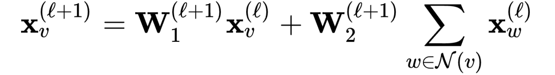
from torch_geometric.nn import GraphConv
class GNN(torch.nn.Module):    def __init__(self, hidden_channels):        super(GNN, self).__init__()        torch.manual_seed(12345)        self.conv1 = GraphConv(dataset.num_node_features, hidden_channels)        self.conv2 = GraphConv(hidden_channels, hidden_channels)        self.conv3 = GraphConv(hidden_channels, hidden_channels)        self.lin = Linear(hidden_channels, dataset.num_classes)
    def forward(self, x, edge_index, batch):        x = self.conv1(x, edge_index)        x = x.relu()        x = self.conv2(x, edge_index)        x = x.relu()        x = self.conv3(x, edge_index)
        x = global_mean_pool(x, batch)
        x = F.dropout(x, p=0.5, training=self.training)        x = self.lin(x)                return x
model = GNN(hidden_channels=64)print(model)
GNN(  (conv1): GraphConv(7, 64)  (conv2): GraphConv(64, 64)  (conv3): GraphConv(64, 64)  (lin): Linear(in_features=64, out_features=2, bias=True))
model = GNN(hidden_channels=64)print(model)optimizer = torch.optim.Adam(model.parameters(), lr=0.01)
for epoch in range(1, 201):    train()    train_acc = test(train_loader)    test_acc = test(test_loader)    print(f'Epoch: {epoch:03d}, Train Acc: {train_acc:.4f}, Test Acc: {test_acc:.4f}')# 输出结果GNN(  (conv1): GraphConv(7, 64)  (conv2): GraphConv(64, 64)  (conv3): GraphConv(64, 64)  (lin): Linear(in_features=64, out_features=2, bias=True))...省略结果输出Epoch: 191, Train Acc: 0.9467, Test Acc: 0.8421Epoch: 192, Train Acc: 0.9467, Test Acc: 0.8421Epoch: 193, Train Acc: 0.9467, Test Acc: 0.8158Epoch: 194, Train Acc: 0.9400, Test Acc: 0.8421Epoch: 195, Train Acc: 0.9467, Test Acc: 0.8421Epoch: 196, Train Acc: 0.9467, Test Acc: 0.8421Epoch: 197, Train Acc: 0.9467, Test Acc: 0.8421Epoch: 198, Train Acc: 0.9467, Test Acc: 0.8421Epoch: 199, Train Acc: 0.9467, Test Acc: 0.8421Epoch: 200, Train Acc: 0.9467, Test Acc: 0.8421

04

总结

这一节主要学习了

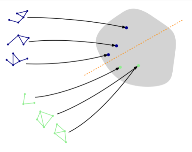
• 将GNN应用到图分类任务上
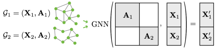
• 图数据的批处理
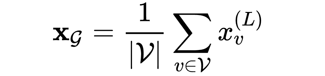
• 使用readout layer获得图的嵌入