【Code】GraphSAGE 源码解析

1.GraphSAGE
本文代码源于 DGL 的 Example 的,感兴趣可以去 github 上面查看。
阅读代码的本意是加深对论文的理解,其次是看下大佬们实现算法的一些方式方法。当然,在阅读 GraphSAGE 代码时我也发现了之前忽视的 GraphSAGE 的细节问题和一些理解错误。比如说:之前忽视了 GraphSAGE 的四种聚合方式的具体实现,对 Alogrithm 2 的算法理解也有问题,再回头看那篇 GraphSAGE 的推文时,实在惨不忍睹= =。
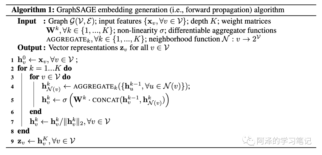
进入正题,简单回顾一下 GraphSAGE。
核心算法:
2.SAGEConv
dgl 已经实现了 SAGEConv 层,所以我们可以直接导入。
有了 SAGEConv 层后,GraphSAGE 实现起来就比较简单。
和基于 GraphConv 实现 GCN 的唯一区别在于把 GraphConv 改成了 SAGEConv:
class GraphSAGE(nn.Module):
    def __init__(self,
                 g,
                 in_feats,
                 n_hidden,
                 n_classes,
                 n_layers,
                 activation,
                 dropout,
                 aggregator_type):
        super(GraphSAGE, self).__init__()
        self.layers = nn.ModuleList()
        self.g = g
        # input layer
        self.layers.append(SAGEConv(in_feats, n_hidden, aggregator_type,
                                    feat_drop=dropout, activation=activation))
        # hidden layers
        for i in range(n_layers - 1):
            self.layers.append(SAGEConv(n_hidden, n_hidden, aggregator_type,
                                        feat_drop=dropout, activation=activation))
        # output layer
        self.layers.append(SAGEConv(n_hidden, n_classes, aggregator_type,
                                    feat_drop=dropout, activation=None)) # activation None

    def forward(self, features):
        h = features
        for layer in self.layers:
            h = layer(self.g, h)
        return h
来看一下 SAGEConv 是如何实现的
SAGEConv 接收七个参数:
-
in_feat:输入的特征大小,可以是一个整型数,也可以是两个整型数。如果用在单向二部图上,则可以用整型数来分别表示源节点和目的节点的特征大小,如果只给一个的话,则默认源节点和目的节点的特征大小一致。需要注意的是,如果参数 aggregator_type 为 gcn 的话,则源节点和目的节点的特征大小必须一致; -
out_feats:输出特征大小; -
aggregator_type:聚合类型,目前支持 mean、gcn、pool、lstm,比论文多一个 gcn 聚合,gcn 聚合可以理解为周围所有的邻居结合和当前节点的均值; -
feat_drop=0.:特征 drop 的概率,默认为 0; -
bias=True:输出层的 bias,默认为 True; -
norm=None:归一化,可以选择一个归一化的方式,默认为 None -
activation=None:激活函数,可以选择一个激活函数去更新节点特征,默认为 None。
class SAGEConv(nn.Module):


    def __init__(self,
                 in_feats,
                 out_feats,
                 aggregator_type,
                 feat_drop=0.,
                 bias=True,
                 norm=None,
                 activation=None):
        super(SAGEConv, self).__init__()

        # expand_as_pair 函数可以返回一个二维元组。
        self._in_src_feats, self._in_dst_feats = expand_as_pair(in_feats)
        self._out_feats = out_feats
        self._aggre_type = aggregator_type
        self.norm = norm
        self.feat_drop = nn.Dropout(feat_drop)
        self.activation = activation
        # aggregator type: mean/pool/lstm/gcn
        if aggregator_type == 'pool':
            self.fc_pool = nn.Linear(self._in_src_feats, self._in_src_feats)
        if aggregator_type == 'lstm':
            self.lstm = nn.LSTM(self._in_src_feats, self._in_src_feats, batch_first=True)
        if aggregator_type != 'gcn':
            self.fc_self = nn.Linear(self._in_dst_feats, out_feats, bias=bias)
        self.fc_neigh = nn.Linear(self._in_src_feats, out_feats, bias=bias)
        self.reset_parameters()

    def reset_parameters(self):
        """初始化参数
        这里的 gain 可以从 calculate_gain 中获取针对非线形激活函数的建议的值
        用于初始化参数
        """
        gain = nn.init.calculate_gain('relu')
        if self._aggre_type == 'pool':
            nn.init.xavier_uniform_(self.fc_pool.weight, gain=gain)
        if self._aggre_type == 'lstm':
            self.lstm.reset_parameters()
        if self._aggre_type != 'gcn':
            nn.init.xavier_uniform_(self.fc_self.weight, gain=gain)
        nn.init.xavier_uniform_(self.fc_neigh.weight, gain=gain)

    def _lstm_reducer(self, nodes):
        """LSTM reducer
        NOTE(zihao): lstm reducer with default schedule (degree bucketing)
        is slow, we could accelerate this with degree padding in the future.
        """
        m = nodes.mailbox['m'] # (B, L, D)
        batch_size = m.shape[0]
        h = (m.new_zeros((1, batch_size, self._in_src_feats)),
             m.new_zeros((1, batch_size, self._in_src_feats)))
        _, (rst, _) = self.lstm(m, h)
        return {'neigh': rst.squeeze(0)}

    def forward(self, graph, feat):
        """ SAGE 层的前向传播
        接收 DGLGraph 和 Tensor 格式的节点特征
        """
        # local_var 会返回一个作用在内部函数中使用的 Graph 对象
        # 外部数据的变化不会影响到这个 Graph
        # 可以理解为保护数据不被意外修改
        graph = graph.local_var()

        if isinstance(feat, tuple):
            feat_src = self.feat_drop(feat[0])
            feat_dst = self.feat_drop(feat[1])
        else:
            feat_src = feat_dst = self.feat_drop(feat)

        h_self = feat_dst

        # 根据不同的聚合类型选择不同的聚合方式
        # 值得注意的是,论文在 3.3 节只给出了三种聚合方式
        # 而这里却多出来一个 gcn 聚合
        # 具体原因将在后文给出
        if self._aggre_type == 'mean':
            graph.srcdata['h'] = feat_src
            graph.update_all(fn.copy_src('h', 'm'), fn.mean('m', 'neigh'))
            h_neigh = graph.dstdata['neigh']
        elif self._aggre_type == 'gcn':
            # check_eq_shape 用于检查源节点和目的节点的特征大小是否一致
            check_eq_shape(feat)
            graph.srcdata['h'] = feat_src
            graph.dstdata['h'] = feat_dst     # same as above if homogeneous
            graph.update_all(fn.copy_src('h', 'm'), fn.sum('m', 'neigh'))
            # divide in_degrees
            degs = graph.in_degrees().to(feat_dst)
            h_neigh = (graph.dstdata['neigh'] + graph.dstdata['h']) / (degs.unsqueeze(-1) + 1)
        elif self._aggre_type == 'pool':
            graph.srcdata['h'] = F.relu(self.fc_pool(feat_src))
            graph.update_all(fn.copy_src('h', 'm'), fn.max('m', 'neigh'))
            h_neigh = graph.dstdata['neigh']
        elif self._aggre_type == 'lstm':
            graph.srcdata['h'] = feat_src
            graph.update_all(fn.copy_src('h', 'm'), self._lstm_reducer)
            h_neigh = graph.dstdata['neigh']
        else:
            raise KeyError('Aggregator type {} not recognized.'.format(self._aggre_type))

        # GraphSAGE GCN does not require fc_self.
        if self._aggre_type == 'gcn':
            rst = self.fc_neigh(h_neigh)
        else:
            rst = self.fc_self(h_self) + self.fc_neigh(h_neigh)
        # activation
        if self.activation is not None:
            rst = self.activation(rst)
        # normalization
        if self.norm is not None:
            rst = self.norm(rst)
        return rst
reset_parameters 函数那里有一个 gain,初始化参数服从 Xavier 均匀分布:
2.1 Aggregate
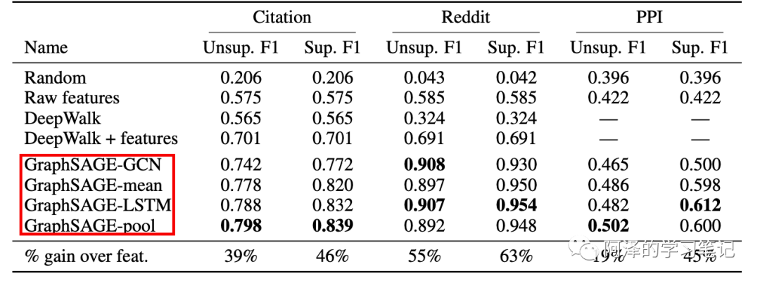
仔细阅读论文时会发现,在实验部分作者给出了四种方式的聚合方法:
配合着论文,我们来阅读下代码
-
mean:mean 聚合首先会对邻居节点进行均值聚合,然后当前节点特征与邻居节点特征该分别送入全连接网络后相加得到结果,对应伪代码如下:
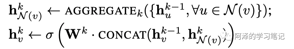
对应代码如下:
h_self = feat_dst
graph.srcdata['h'] = feat_src
graph.update_all(fn.copy_src('h', 'm'), fn.mean('m', 'neigh'))
h_neigh = graph.dstdata['neigh']
rst = self.fc_self(h_self) + self.fc_neigh(h_neigh)
-
gcn:gcn 聚合首先对邻居节点的特征和自身节点的特征求均值,得到的聚合特征送入到全连接网络中,对应论文公式如下:
对应代码如下:
graph.srcdata['h'] = feat_src
graph.dstdata['h'] = feat_dst
graph.update_all(fn.copy_src('h', 'm'), fn.sum('m', 'neigh'))
# divide in_degrees
degs = graph.in_degrees().to(feat_dst)
h_neigh = (graph.dstdata['neigh'] + graph.dstdata['h']) / (degs.unsqueeze(-1) + 1)
rst = self.fc_neigh(h_neigh)
gcn 与 mean 的关键区别在于节点邻居节点和当前节点取平均的方式:gcn 是直接将当前节点和邻居节点取平均,而 mean 聚合是 concat 当前节点的特征和邻居节点的特征,所以「前者只经过一个全连接层,而后者是分别经过全连接层」。
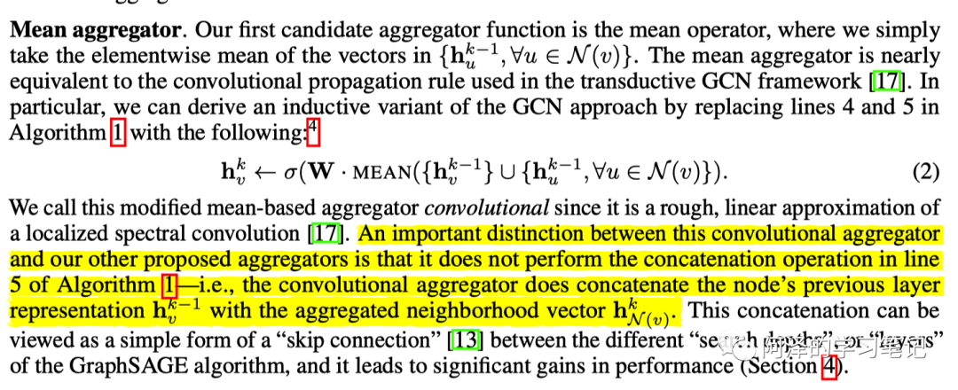
这里利用下斯坦福大学的同学实现的 GCN 聚合器的解释,如果不明白的话,可以去其 github 仓库查看源码:
class MeanAggregator(Layer):
    """
    Aggregates via mean followed by matmul and non-linearity.
    """

class GCNAggregator(Layer):
    """
    Aggregates via mean followed by matmul and non-linearity.
    Same matmul parameters are used self vector and neighbor vectors.
    """
-
pool:池化方法中,每一个节点的向量都会对应一个全连接神经网络,然后基于 elementwise 取最大池化操作。对应公式如下:
对应代码如下:
    graph.srcdata['h'] = F.relu(self.fc_pool(feat_src))
    graph.update_all(fn.copy_src('h', 'm'), fn.max('m', 'neigh'))
    h_neigh = graph.dstdata['neigh']
-
lstm:LSTM 聚合器,其表达能力比 mean 聚合器要强,但是 LSTM 是非对称的,即其考虑节点的顺序性,论文作者通过将节点进行随机排列来调整 LSTM 对无序集的支持。
    def _lstm_reducer(self, nodes):
        """LSTM reducer
        m = nodes.mailbox['m'] # (B, L, D)
        batch_size = m.shape[0]
        h = (m.new_zeros((1, batch_size, self._in_src_feats)),
             m.new_zeros((1, batch_size, self._in_src_feats)))
        _, (rst, _) = self.lstm(m, h)
        return {'neigh': rst.squeeze(0)}

    graph.srcdata['h'] = feat_src
    graph.update_all(fn.copy_src('h', 'm'), self._lstm_reducer)
    h_neigh = graph.dstdata['neigh']
以上便是利用 SAGEConv 实现 GraphSAGE 的方法,剩余训练的内容与前文介绍 GCN 一直,不再进行介绍。
3.Neighbor sampler
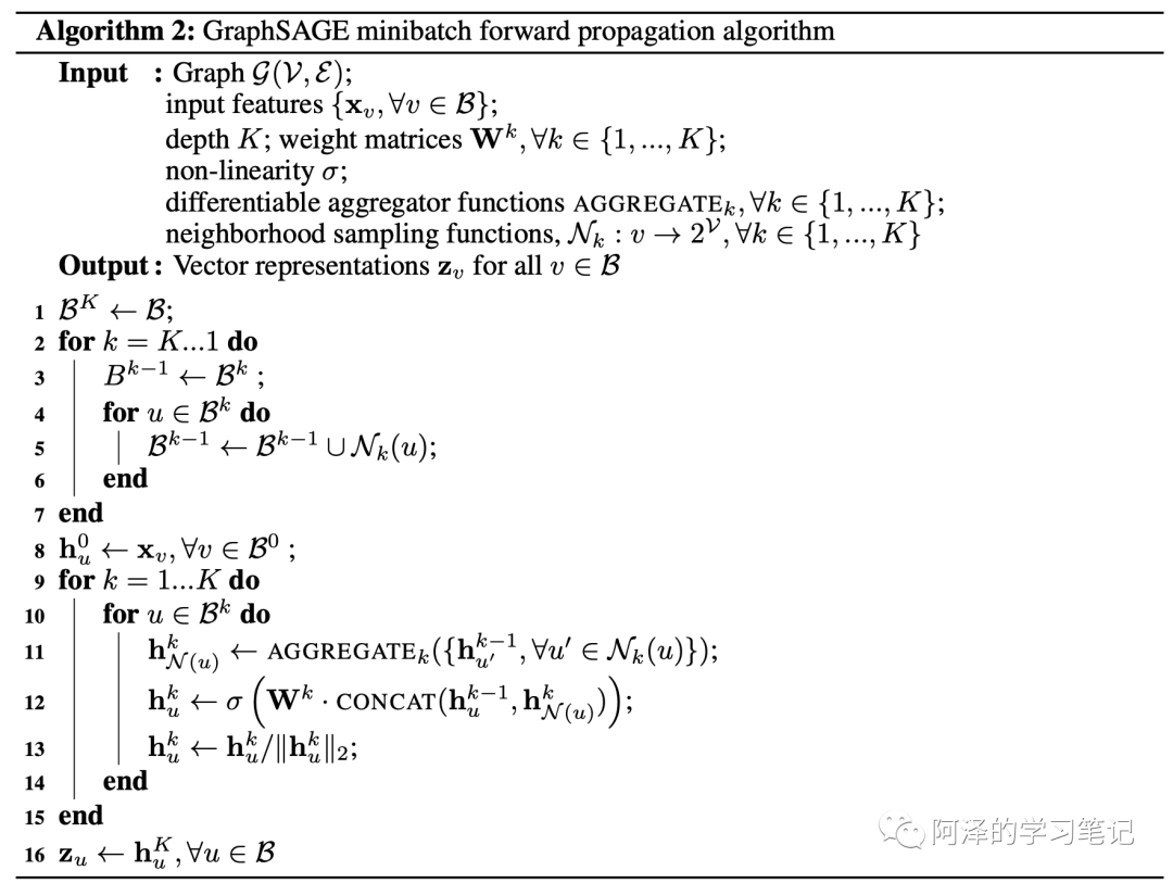
这里再介绍一下基于节点邻居采样并利用 minibatch 的方法进行前向传播的 GraphSAGE 的实现。
这种方法适用于大图,并且能够并行计算。
import dgl
import numpy as np
import torch as th
import torch.nn as nn
import torch.nn.functional as F
import torch.optim as optim
from torch.utils.data import DataLoader
from dgl.nn import SAGEConv
import time
from dgl.data import RedditDataset
import tqdm
class NeighborSampler(object):
    """
    对应 Algorithm 2 算法的 1-7 步,配合 PinSAGE 理解会更容易些
    """

    def __init__(self, g, fanouts):
        """
        g 为 DGLGraph;
        fanouts 为采样节点的数量,实验使用 10,25,指一阶邻居采样 10 个,二阶邻居采样 25 个。
        """
        self.g = g
        self.fanouts = fanouts

    def sample_blocks(self, seeds):
        seeds = th.LongTensor(np.asarray(seeds))
        blocks = []
        for fanout in self.fanouts:
            # sample_neighbors 可以对每一个种子的节点进行邻居采样并返回相应的子图
            # replace=True 表示用采样后的邻居节点代替所有邻居节点
            frontier = dgl.sampling.sample_neighbors(g, seeds, fanout, replace=True)
            # 将图转变为可以用于消息传递的二部图(源节点和目的节点)
            # 其中源节点的 id 也包含目的节点的 id
            # 主要是为了方便进行消息传递,类似 PinSAGE 的做法
            block = dgl.to_block(frontier, seeds)
            # 获取新图的源节点作为种子节点,为下一层作准备
            seeds = block.srcdata[dgl.NID]
            # 把这一层放在最前面,因为这是一个逆向操作。
            blocks.insert(0, block)
        return blocks
Algorithm 2 伪代码如下所示:
# GraphSAGE 的代码实现
class GraphSAGE(nn.Module):
    def __init__(self,
                 in_feats,
                 n_hidden,
                 n_classes,
                 n_layers,
                 activation,
                 dropout):
        super().__init__()
        self.n_layers = n_layers
        self.n_hidden = n_hidden
        self.n_classes = n_classes
        self.layers = nn.ModuleList()
        self.layers.append(SAGEConv(in_feats, n_hidden, 'mean'))
        for i in range(1, n_layers - 1):
            self.layers.append(dglnn.SAGEConv(n_hidden, n_hidden, 'mean'))
        self.layers.append(SAGEConv(n_hidden, n_classes, 'mean'))
        self.dropout = nn.Dropout(dropout)
        self.activation = activation

    def forward(self, blocks, x):
        # block 是我们采样获得的二部图,这里用于传播消息
        h = x
        for l, (layer, block) in enumerate(zip(self.layers, blocks)):
            h_dst = h[:block.number_of_dst_nodes()]
            h = layer(block, (h, h_dst))
            if l != len(self.layers) - 1:
                h = self.activation(h)
                h = self.dropout(h)
        return h

    def inference(self, g, x, batch_size, device):
        # 用于评估,针对的是完全图
        # 目前会出现重复计算的问题,优化方案还在 to do list 上
        nodes = th.arange(g.number_of_nodes())
        for l, layer in enumerate(self.layers):
            y = th.zeros(g.number_of_nodes(), self.n_hidden if l != len(self.layers) - 1 else self.n_classes)
            for start in tqdm.trange(0, len(nodes), batch_size):
                end = start + batch_size
                batch_nodes = nodes[start:end]
                block = dgl.to_block(dgl.in_subgraph(g, batch_nodes), batch_nodes)
                input_nodes = block.srcdata[dgl.NID]

                h = x[input_nodes].to(device)
                h_dst = h[:block.number_of_dst_nodes()]
                h = layer(block, (h, h_dst))
                if l != len(self.layers) - 1:
                    h = self.activation(h)
                    h = self.dropout(h)
                y[start:end] = h.cpu()
            x = y
        return y
def prepare_mp(g):
    """
    一种临时的异构图内存解决方案
    """
    g.in_degree(0)
    g.out_degree(0)
    g.find_edges([0])

def compute_acc(pred, labels):
    """
    计算的准确率
    """
    return (th.argmax(pred, dim=1) == labels).float().sum() / len(pred)

def evaluate(model, g, inputs, labels, val_mask, batch_size, device):
    """
    评估模型
    """
    model.eval()
    with th.no_grad():
        pred = model.inference(g, inputs, batch_size, device)
    model.train()
    return compute_acc(pred[val_mask], labels[val_mask])

def load_subtensor(g, labels, seeds, input_nodes, device):
    """
    将一组节点的特征和标签复制到 GPU 上。
    """
    batch_inputs = g.ndata['features'][input_nodes].to(device)
    batch_labels = labels[seeds].to(device)
    return batch_inputs, batch_labels
gpu = -1
num_epochs = 20
num_hidden = 16
num_layers = 2
fan_out = '10,25'
batch_size = 1000
log_every = 20
eval_every = 5
lr = 0.003
dropout = 0.5
num_workers = 0

if gpu >= 0:
    device = th.device('cuda:%d' % gpu)
else:
    device = th.device('cpu')

# load reddit data
data = RedditDataset(self_loop=True)
train_mask = data.train_mask
val_mask = data.val_mask
features = th.Tensor(data.features)
in_feats = features.shape[1]
labels = th.LongTensor(data.labels)
n_classes = data.num_labels
# Construct graph
g = dgl.graph(data.graph.all_edges())
g.ndata['features'] = features
prepare_mp(g)
Finished data loading.
  NumNodes: 232965
  NumEdges: 114848857
  NumFeats: 602
  NumClasses: 41
  NumTrainingSamples: 153431
  NumValidationSamples: 23831
  NumTestSamples: 55703
开始训练:
train_nid = th.LongTensor(np.nonzero(train_mask)[0])
val_nid = th.LongTensor(np.nonzero(val_mask)[0])
train_mask = th.BoolTensor(train_mask)
val_mask = th.BoolTensor(val_mask)

# Create sampler
sampler = NeighborSampler(g, [int(fanout) for fanout in fan_out.split(',')])

# Create PyTorch DataLoader for constructing blocks
# collate_fn 参数指定了 sampler,可以对 batch 中的节点进行采样
dataloader = DataLoader(
    dataset=train_nid.numpy(),
    batch_size=batch_size,
    collate_fn=sampler.sample_blocks,
    shuffle=True,
    drop_last=False,
    num_workers=num_workers)

# Define model and optimizer
model = GraphSAGE(in_feats, num_hidden, n_classes, num_layers, F.relu, dropout)
model = model.to(device)
loss_fcn = nn.CrossEntropyLoss()
loss_fcn = loss_fcn.to(device)
optimizer = optim.Adam(model.parameters(), lr=lr)

# Training loop
avg = 0
iter_tput = []
for epoch in range(num_epochs):
    tic = time.time()

    for step, blocks in enumerate(dataloader):
        tic_step = time.time()

        input_nodes = blocks[0].srcdata[dgl.NID]
        seeds = blocks[-1].dstdata[dgl.NID]

        # Load the input features as well as output labels
        batch_inputs, batch_labels = load_subtensor(g, labels, seeds, input_nodes, device)

        # Compute loss and prediction
        batch_pred = model(blocks, batch_inputs)
        loss = loss_fcn(batch_pred, batch_labels)
        optimizer.zero_grad()
        loss.backward()
        optimizer.step()

        iter_tput.append(len(seeds) / (time.time() - tic_step))
        if step % log_every == 0:
            acc = compute_acc(batch_pred, batch_labels)
            gpu_mem_alloc = th.cuda.max_memory_allocated() / 1000000 if th.cuda.is_available() else 0
            print('Epoch {:05d} | Step {:05d} | Loss {:.4f} | Train Acc {:.4f} | Speed (samples/sec) {:.4f} | GPU {:.1f} MiB'.format(
                epoch, step, loss.item(), acc.item(), np.mean(iter_tput[3:]), gpu_mem_alloc))

    toc = time.time()
    print('Epoch Time(s): {:.4f}'.format(toc - tic))
    if epoch >= 5:
        avg += toc - tic
    if epoch % eval_every == 0 and epoch != 0:
        eval_acc = evaluate(model, g, g.ndata['features'], labels, val_mask, batch_size, device)
        print('Eval Acc {:.4f}'.format(eval_acc))

print('Avg epoch time: {}'.format(avg / (epoch - 4)))
4.Reference
-
Github:dmlc/dgl -
williamleif/GraphSAGE
推荐阅读
征稿启示| 200元稿费+5000DBC(价值20个小时GPU算力)
文本自动摘要任务的“不完全”心得总结番外篇——submodular函数优化
斯坦福大学NLP组Python深度学习自然语言处理工具Stanza试用
太赞了!Springer面向公众开放电子书籍,附65本数学、编程、机器学习、深度学习、数据挖掘、数据科学等书籍链接及打包下载
数学之美中盛赞的 Michael Collins 教授,他的NLP课程要不要收藏?
关于AINLP
AINLP 是一个有趣有AI的自然语言处理社区,专注于 AI、NLP、机器学习、深度学习、推荐算法等相关技术的分享,主题包括文本摘要、智能问答、聊天机器人、机器翻译、自动生成、知识图谱、预训练模型、推荐系统、计算广告、招聘信息、求职经验分享等,欢迎关注!加技术交流群请添加AINLPer(id:ainlper),备注工作/研究方向+加群目的。

阅读至此了,点个在看吧👇