迁移学习不好懂？这里有一个PyTorch项目帮你理解

会员服务 ·

迁移学习不好懂？这里有一个PyTorch项目帮你理解

2019 年 3 月 6 日 新智元

新智元报道

来源：Medium

编辑：元子

【新智元导读】迁移学习是一个非常重要的机器学习技术，已被广泛应用于机器学习的许多应用中。本文的目标是让读者理解迁移学习的意义，了解转学习的重要性，并学会使用PyTorch进行实践。

前几天新智元介绍了在线元学习，以及元奖励学习。元学习有一个非常重要的理念是在较少样本量的情况下，让机器能够自己学会学习。

这一点和迁移学习非常相似。吴恩达曾经说过"迁移学习将会是继监督学习之后的下一个机器学习商业成功的驱动力"。

相比而言，依赖大量数据进行训练的其他机器学习手段（例如昨天新智元报道的GPipe），对数据和算力的依赖有点过于严重。况且，数据和算力那么贵！

迁移学习的一大特色，就是“将一个任务环境中学到的东西用来提升在另一个任务环境中模型的泛化能力”。

没有GPU也没关系，可以使用谷歌的免费GPU服务，通过谷歌Colab来训练模型。

借TensorFlow 2.0发布之际，就让我们对比一下，通过PyTorch来更直观、更深入的了解迁移学习。

前期准备

本次旅程，我们将使用预先训练的网络，来构建用于疟疾检测的图像分类器，这个分类器只需要将得到的数据，分为“感染”“未感染”两类。

我们将要用到的图像数据集可以在这里下载👇

https://drive.google.com/open?id=16DbIOMCtCuRuMdYF64MPv3iLqpSG6tfv

经过预先训练的网络在ImageNet上进行了训练，其中包含120万张1000个类别的图像，

用到的模型是torchvision.models，它有6种不同的架构我们可以使用。

torchvision.models具有模型性能的细分以及可以使用的层数（由模型附带的数字表示）。

加载所有必需的包和库：

%matplotlib inline%config InlineBackend.figure_format = 'retina'from matplotlib import pyplot as pltimport torchfrom torch import nnimport torch.nn.functional as Ffrom torch import optimfrom torch.autograd import Variablefrom torchvision import datasets, transforms, modelsfrom PIL import Imageimport numpy as npimport osfrom torch.utils.data.sampler import SubsetRandomSamplerimport pandas as pd

将数据进行可视化：

img_dir='/content/drive/My Drive/app/cell_images'def imshow(image):    """Display image"""    plt.figure(figsize=(6, 6))    plt.imshow(image)    plt.axis('off')    plt.show()# Example imagex = Image.open(img_dir + '/Parasitized/C33P1thinF_IMG_20150619_114756a_cell_179.png')np.array(x).shapeimshow(x)

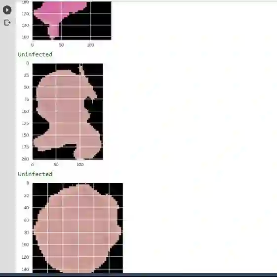
下图是感染的图

定义转换并加载进数据

转换是将一个图形、表达式或函数转换为另一个图形、表达式或函数的过程。

我们需要为训练、测试以及验证数据定义一些转换。值得注意的，可能有的类别图像太少，不够进行转换，为了增加网络识别的图像数量，我们执行所谓的数据增强。

在训练期间，我们随机裁剪、缩放和旋转图像，以便在每个时期，网络会看到同一图像的不同变化，提高实验的准确性。

   # Define your transforms for the training, validation, and testing setstrain_transforms = transforms.Compose([transforms.RandomResizedCrop(size=256, scale=(0.8, 1.0)),                                      transforms.RandomRotation(degrees=15),                                      transforms.ColorJitter(),                                      transforms.RandomHorizontalFlip(),                                      transforms.CenterCrop(size=224),  # Image net standards                                      transforms.ToTensor(),                                      transforms.Normalize([0.485, 0.456, 0.406],                                                           [0.229, 0.224, 0.225])                                      ])
test_transforms = transforms.Compose([transforms.Resize(256),                                      transforms.CenterCrop(224),                                      transforms.ToTensor(),                                      transforms.Normalize([0.485, 0.456, 0.406],                                                            [0.229, 0.224, 0.225])])
validation_transforms = transforms.Compose([transforms.Resize(256),                                            transforms.CenterCrop(224),                                            transforms.ToTensor(),                                            transforms.Normalize([0.485, 0.456, 0.406],                                                                  [0.229, 0.224, 0.225])])                                                           [0.229, 0.224, 0.225])])

接下来加载数据集。最简单的方法是用torchvision的dataset.ImageFolder。

加载imageFolder后，我们将数据拆分为20％验证集和10％测试集; 然后将它传递给DataLoader。

它接收一个类似从ImageFolder获得的数据集，并返回批量图像及其相应的标签（可以将改组设置为true以在时期内引入变化）。

#Loading in the dataset
train_data = datasets.ImageFolder(img_dir,transform=train_transforms)# number of subprocesses to use for data loadingnum_workers = 0# percentage of training set to use as validationvalid_size = 0.2
test_size = 0.1
# obtain training indices that will be used for validationnum_train = len(train_data)indices = list(range(num_train))np.random.shuffle(indices)valid_split = int(np.floor((valid_size) * num_train))test_split = int(np.floor((valid_size+test_size) * num_train))valid_idx, test_idx, train_idx = indices[:valid_split], indices[valid_split:test_split], indices[test_split:]
print(len(valid_idx), len(test_idx), len(train_idx))
# define samplers for obtaining training and validation batchestrain_sampler = SubsetRandomSampler(train_idx)valid_sampler = SubsetRandomSampler(valid_idx)test_sampler = SubsetRandomSampler(test_idx)
# prepare data loaders (combine dataset and sampler)train_loader = torch.utils.data.DataLoader(train_data, batch_size=32,    sampler=train_sampler, num_workers=num_workers)valid_loader = torch.utils.data.DataLoader(train_data, batch_size=32,     sampler=valid_sampler, num_workers=num_workers)test_loader = torch.utils.data.DataLoader(train_data, batch_size=32,     sampler=test_sampler, num_workers=num_workers)

模型训练流程

1. 加载预先训练的模型

device = torch.device("cuda" if torch.cuda.is_available() else "cpu")#pretrained=True will download a pretrained network for usmodel = models.densenet121(pretrained=True)model

PyTorch以及几乎所有其他深度学习框架，都使用CUDA来有效地计算GPU上的前向和后向传递。

在PyTorch中，我们使用model.cuda（）将模型参数和其他张量移动到GPU内存，或者从GPU移回，

2. 冻结卷积层并使用自定义分类器替换完全连接的层

#Freezing model parameters and defining the fully connected network to be attached to the model, loss function and the optimizer.#We there after put the model on the GPUsfor param in model.parameters():  param.require_grad = Falsefc = nn.Sequential(    nn.Linear(1024, 460),    nn.ReLU(),    nn.Dropout(0.4),        nn.Linear(460,2),    nn.LogSoftmax(dim=1)    )model.classifier = fccriterion = nn.NLLLoss()#Over here we want to only update the parameters of the classifier sooptimizer = torch.optim.Adam(model.classifier.parameters(), lr=0.003)model.to(device)

冻结模型参数允许我们为早期卷积层保留预训练模型的权重，其目的是用于特征提取。

然后我们定义我们的全连接网络，他将作为输入神经元，示例代码中是1024，这个数字取决于预训练模型的输入神经元，和自定义隐藏层。

我们还定义了要使用的激活函数，和有助于通过随机关闭层中的神经元，以强制在剩余节点之间共享信息，来避免过度拟合的丢失。

在我们定义了自定义全连接网络之后，我们将其连接到预先训练好的模型的完全连接网络。

接下来我们定义损失函数，优化器，并通过将模型移动到GPU来准备训练模型。

3. 为特定任务训练自定义分类器

在训练期间，我们遍历每个时期的DataLoader。对于每个batch，使用标准函数计算损失。使用loss.backward（）方法计算相对于模型参数的损失梯度。

optimizer.zero_grad（）负责清除任何累积的梯度，因为我们会一遍又一遍地计算梯度。

optimizer.step（）使用具有动量的随机梯度下降（Adam）更新模型参数。

为了防止过度拟合，我们使用一种称为早期停止的强大技术。背后的想法很简单，当验证数据集上的性能开始降低时停止训练。

#Training the model and saving checkpoints of best performances. That is lower validation loss and higher accuracyepochs = 10valid_loss_min = np.Infimport timefor epoch in range(epochs):        start = time.time()        #scheduler.step()    model.train()        train_loss = 0.0    valid_loss = 0.0        for inputs, labels in train_loader:                       # Move input and label tensors to the default device        inputs, labels = inputs.to(device), labels.to(device)                optimizer.zero_grad()                logps = model(inputs)        loss = criterion(logps, labels)        loss.backward()        optimizer.step()train_loss += loss.item()                   model.eval()        with torch.no_grad():        accuracy = 0        for inputs, labels in valid_loader:                        inputs, labels = inputs.to(device), labels.to(device)            logps = model.forward(inputs)            batch_loss = criterion(logps, labels)valid_loss += batch_loss.item()# Calculate accuracy            ps = torch.exp(logps)            top_p, top_class = ps.topk(1, dim=1)            equals = top_class == labels.view(*top_class.shape)            accuracy += torch.mean(equals.type(torch.FloatTensor)).item()                                            # calculate average losses    train_loss = train_loss/len(train_loader)    valid_loss = valid_loss/len(valid_loader)    valid_accuracy = accuracy/len(valid_loader)           # print training/validation statistics     print('Epoch: {} \tTraining Loss: {:.6f} \tValidation Loss: {:.6f} \tValidation Accuracy: {:.6f}'.format(        epoch + 1, train_loss, valid_loss, valid_accuracy))                        if valid_loss <= valid_loss_min:                  print('Validation loss decreased ({:.6f} --> {:.6f}).  Saving model ...'.format(      valid_loss_min,      valid_loss))      model_save_name = "Malaria.pt"      path = F"/content/drive/My Drive/{model_save_name}"torch.save(model.state_dict(), path)      valid_loss_min = valid_loss                   print(f"Time per epoch: {(time.time() - start):.3f} seconds")

在耐心地等待训练过程完成并保存最佳模型参数的检查点之后，让我们加载检查点并在看不见的数据（测试数据）上测试模型的性能。

从磁盘加载已保存的模型

model.load_state_dict(torch.load('Malaria.pt'))

在看不见的数据上测试加载的模型。我们对看不见的数据有90％的准确率，这在第一次尝试时非常令人印象深刻。

def test(model, criterion):# monitor test loss and accuracy    test_loss = 0.    correct = 0.    total = 0.for batch_idx, (data, target) in enumerate(test_loader):        # move to GPU        if torch.cuda.is_available():            data, target = data.cuda(), target.cuda()        # forward pass: compute predicted outputs by passing inputs to the model        output = model(data)        # calculate the loss        loss = criterion(output, target)        # update average test loss         test_loss = test_loss + ((1 / (batch_idx + 1)) * (loss.data - test_loss))        # convert output probabilities to predicted class        pred = output.data.max(1, keepdim=True)[1]        # compare predictions to true label        correct += np.sum(np.squeeze(pred.eq(target.data.view_as(pred))).cpu().numpy())        total += data.size(0)                print('Test Loss: {:.6f}\n'.format(test_loss))print('\nTest Accuracy: %2d%% (%2d/%2d)' % (        100. * correct / total, correct, total))test(model, criterion)Test Loss: 0.257728   Test Accuracy: 90% (2483/2756)

现在我们对模型有了信心，现在是时候进行一些预测并将结果可视化了。

def load_input_image(img_path):        image = Image.open(img_path)    prediction_transform = transforms.Compose([transforms.Resize(size=(224, 224)),                                     transforms.ToTensor(),                                      transforms.Normalize([0.485, 0.456, 0.406],                                                           [0.229, 0.224, 0.225])])
    # discard the transparent, alpha channel (that's the :3) and add the batch dimension    image = prediction_transform(image)[:3,:,:].unsqueeze(0)    return image

def predict_malaria(model, class_names, img_path):    # load the image and return the predicted breed    img = load_input_image(img_path)    model = model.cpu()    model.eval()    idx = torch.argmax(model(img))    return class_names[idx]

from glob import globfrom PIL import Imagefrom termcolor import colored
class_names=['Parasitized','Uninfected']inf = np.array(glob(img_dir + "/Parasitized/*"))uninf = np.array(glob(img_dir + "/Uninfected/*"))for i in range(3):    img_path=inf[i]    img = Image.open(img_path)    if predict_malaria(model, class_names, img_path) == 'Parasitized':        print(colored('Parasitized', 'green'))    else:        print(colored('Uninfected', 'red'))    plt.imshow(img)    plt.show()for i in range(3):    img_path=uninf[i]    img = Image.open(img_path)    if predict_malaria(model, class_names, img_path) == 'Uninfected':        print(colored('Uninfected', 'green'))    else:        print(colored('Parasitized', 'red'))            plt.imshow(img)    plt.show()