【原】Coursera—Andrew Ng机器学习—编程作业 Programming Exercise 2——逻辑回归
作业说明
Exercise 2,Week 3,使用Octave实现逻辑回归模型。数据集 ex2data1.txt ,ex2data2.txt
实现 Sigmoid 、代价函数计算Computing Cost 和 梯度下降Gradient Descent。

文件清单
- ex2.m - Octave/MATLAB script that steps you through the exercise
- ex2 reg.m - Octave/MATLAB script for the later parts of the exercise
- ex2data1.txt - Training set for the first half of the exercise
- ex2data2.txt - Training set for the second half of the exercise
- submit.m - Submission script that sends your solutions to our servers
- mapFeature.m - Function to generate polynomial features
- plotDecisionBoundary.m - Function to plot classifier’s decision boundary
- [*] plotData.m - Function to plot 2D classification data
- [*] sigmoid.m - Sigmoid Function
- [*] costFunction.m - Logistic Regression Cost Function
- [*] predict.m - Logistic Regression Prediction Function
- [*] costFunctionReg.m - Regularized Logistic Regression Cost
* 为必须要完成的
结论
正则化不涉及第一个 θ0
逻辑回归
背景:大学管理员,想要根据两门课的历史成绩记录来每个是否被允许入学。
ex2data1.txt ,前两列是两门课的成绩,第三列是y值 0 和 1。
一、绘制数据图
plotData.m:
1   positive = find(y == 1);
2   negative = find(y == 0);
3
4   plot(X(positive,1),X(positive,2),'k+','MarkerFaceColor','g',
5     'MarkerSize',7);
6   hold on;
7   plot(X(negative,1),X(negative,2),'ko','MarkerFaceColor','y',
8     'MarkerSize',7);
运行效果如下:

二、sigmoid 函数
1 function g = sigmoid(z)
2 % Instructions: Compute the sigmoid of each value of z (z can be a matrix,
3 %               vector or scalar).
4   g = 1 ./ (1 + exp(-z));
5 end
三、代价函数
costFunction.m:
 1 function [J, grad] = costFunction(theta, X, y)
 2
 3   m = length(y); % number of training examples
 4
 5   part1 = -1 * y' * log(sigmoid(X * theta));
 6   part2 = (1 - y)' * log(1 - sigmoid(X * theta));
 7   J = 1 / m * (part1 - part2);
 8
 9   grad = 1 / m * X' *((sigmoid(X * theta) - y));
10
11 end
四、预测函数
输入X和theta,返回预测结果向量。每个值是 0 或 1
 1 function p = predict(theta, X)
 2 %PREDICT Predict whether the label is 0 or 1 using learned logistic
 3 %regression parameters theta
 4 %   p = PREDICT(theta, X) computes the predictions for X using a
 5 %   threshold at 0.5 (i.e., if sigmoid(theta'*x) >= 0.5, predict 1)
 6
 7 m = size(X, 1); % Number of training examples
 8
 9 % 最开始没有四舍五入,导致错误
10 p = round(sigmoid(X * theta));
11
12 end
五、进行逻辑回归
ex1.m 中的调用:
加载数据:
1 data = load('ex2data1.txt');
2 X = data(:, [1, 2]); y = data(:, 3);
3
4 [m, n] = size(X);
5
6 % Add intercept term to x and X_test
7 X = [ones(m, 1) X];
8
9 initial_theta = zeros(n + 1, 1);
调用 fminunc 函数
1 options = optimset('GradObj', 'on', 'MaxIter', 400);
2 [theta, cost] = ...
3     fminunc(@(t)(costFunction(t, X, y)), initial_theta, options);
四、绘制边界线
plotDecisionBoundary.m
function plotDecisionBoundary(theta, X, y)
%PLOTDECISIONBOUNDARY Plots the data points X and y into a new figure with
%the decision boundary defined by theta
%   PLOTDECISIONBOUNDARY(theta, X,y) plots the data points with + for the
%   positive examples and o for the negative examples. X is assumed to be
%   a either
%   1) Mx3 matrix, where the first column is an all-ones column for the
%      intercept.
%   2) MxN, N>3 matrix, where the first column is all-ones

% Plot Data
plotData(X(:,2:3), y);
hold on

if size(X, 2) <= 3
    % Only need 2 points to define a line, so choose two endpoints
    plot_x = [min(X(:,2))-2,  max(X(:,2))+2];

    % Calculate the decision boundary line
    plot_y = (-1./theta(3)).*(theta(2).*plot_x + theta(1));

    % Plot, and adjust axes for better viewing
    plot(plot_x, plot_y)

    % Legend, specific for the exercise
    legend('Admitted', 'Not admitted', 'Decision Boundary')
    axis([30, 100, 30, 100])
else
    % Here is the grid range
    u = linspace(-1, 1.5, 50);
    v = linspace(-1, 1.5, 50);

    z = zeros(length(u), length(v));
    % Evaluate z = theta*x over the grid
    for i = 1:length(u)
        for j = 1:length(v)
            z(i,j) = mapFeature(u(i), v(j))*theta;
        end
    end
    z = z'; % important to transpose z before calling contour

    % Plot z = 0
    % Notice you need to specify the range [0, 0]
    contour(u, v, z, [0, 0], 'LineWidth', 2)
end
hold off

end

正则化逻辑回归
背景:预测来自制造工厂的微芯片是否通过质量保证(QA)。 在QA期间,每个微芯片都经过两个测试以确保其正常运行。
ex2data2.txt ,前两列是测试结果的成绩,第三列是y值 0 和 1。
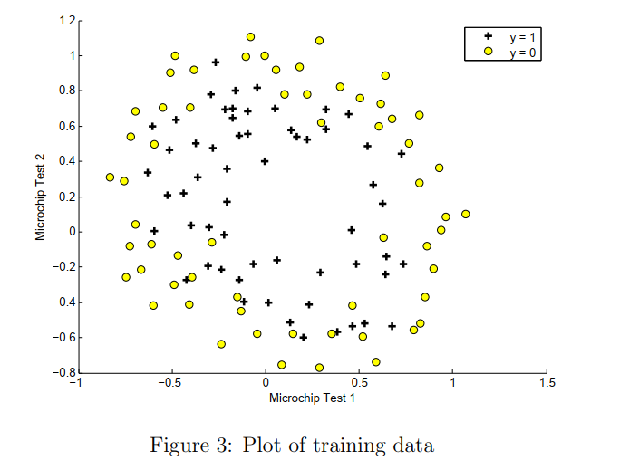
只有两个feature,使用直线不能划分。
为了让数据拟合的更好,使用mapFeature函数,将x1,x2两个feature扩展到六次方。
六次方曲线复杂,容易造成过拟合,所以需要正则化。
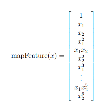
mapFeature.m
 1 function out = mapFeature(X1, X2)
 2 % MAPFEATURE Feature mapping function to polynomial features
 3 %
 4 %   MAPFEATURE(X1, X2) maps the two input features
 5 %   to quadratic features used in the regularization exercise.
 6 %
 7 %   Returns a new feature array with more features, comprising of
 8 %   X1, X2, X1.^2, X2.^2, X1*X2, X1*X2.^2, etc..
 9 %
10 %   Inputs X1, X2 must be the same size
11 %
12
13 degree = 6;
14 out = ones(size(X1(:,1)));
15 for i = 1:degree
16     for j = 0:i
17         out(:, end+1) = (X1.^(i-j)).*(X2.^j);
18     end
19 end
20
21 end
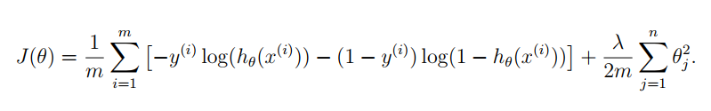
二、代价函数
注意:θ0不参与正则化。
正则化逻辑回归的代价函数如下,分为三项:
梯度下降算法如下:


coatFunctionReg.m 如下:
function [J, grad] = costFunctionReg(theta, X, y, lambda)
  m = length(y); % number of training examples

  % theta0 不参与正则化。直接让变量等于theta,将第一个元素置为0,再参与和 λ 的运算
  t = theta;  t(1) = 0;

  % 第一项
  part1 = -y' * log(sigmoid(X * theta));
  % 第二项
  part2 = (1 - y)' * log(1 - sigmoid(X * theta));

  % 正则项
  regTerm = lambda / 2 / m * t' * t;
  J = 1 / m * (part1 - part2) + regTerm;

  % 梯度
  grad = 1 / m * X' *((sigmoid(X * theta) - y)) + lambda / m * t;

end
em2_reg.m 里的调用
% 加载数据
data = load('ex2data2.txt');
X = data(:, [1, 2]); y = data(:, 3);

% mapfeature
X = mapFeature(X(:,1), X(:,2));

% Initialize fitting parameters
initial_theta = zeros(size(X, 2), 1);
lambda = 1;

% 调用 fminunc方法
options = optimset('GradObj', 'on', 'MaxIter', 400);
[theta, J, exit_flag] = ...
    fminunc(@(t)(costFunctionReg(t, X, y, lambda)), initial_theta, options);
三、参数调整
(1)使用正则化之前,决策边界曲线如下,可以看到存在过拟合现象:
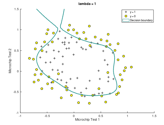
(2)当 λ = 1,决策边界曲线如下。此时训练集预测准确率为 83.05%

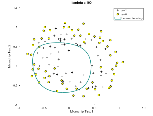
(3)当 λ = 100,曲线如下。此时训练集预测准确率为 61.01%
https://github.com/madoubao/coursera_machine_learning/tree/master/homework/machine-learning-ex2/ex2

